First published:
Journal of Creation
19(1):113–125
April 2005

Browse this issue

Subscribe to Journal of Creation

Cost theory and the cost of substitution—a clarification

by Walter J. ReMine

Figure 1. A simple scenario showing the cost of substitution. Four elephants are the initial new-type. One generation later, five elephants are the new-type. For that to be plausible, a reproduction rate of at least 1.25 (= 5/4) is required in that generation.

J.B.S. Haldane¹ first described the ‘cost of substitution’ and its limitation on the speed of evolution. That gave rise to a problem (see, for example, Dodson²), known today as Haldane’s Dilemma. The problem is more severe in organisms with low reproduction rate and long generation time, such as the higher vertebrates: elephants, whales, apes and humans, etc. Evolutionary geneticists saw this as a compelling issue. Maynard-Smith³ and Kimura⁴ each cited it as the main reason for their revolutionary new views of evolutionary process. Yet the fundamental cost concept fell into long-lived confusion, which limited its deployment. Today, most commentators say the problem is solved, but exhibit little agreement as to why. One modern authority, George C. Williams,⁵ asserted, ‘the [Haldane’s Dilemma] problem was never solved, by Wallace or anyone else’. This paper will show the problem cannot be solved so long as confusion prevails over the fundamentals.

This paper clarifies the cost concept and re-establishes it as a vital tool for investigating population phenomena and our attempts to explain or describe them (herein called scenarios). A cost, as here defined, is simply the reproduction rate required by a given scenario. If the given species cannot supply that reproduction rate, then the scenario is not plausible. In more concise wording, the species ‘cannot pay the cost’. At its core, a cost argument is that simple. A cost and its payment are both reproduction rates. They are defined identically, except that a cost is required by a given scenario, whereas a payment is actually produced within the given species.

Historically, much confusion was created from overemphasizing secondary matters—such as genetic death, the previous organisms that are eliminated, the environment, fitness and genetics. So keep in mind, a cost is about the required reproduction rate, and all else is secondary. Indeed, the unit of cost is reproduction rate (i.e. offspring per individual per generation). Every cost is specified in terms of reproduction rate. This also means every cost is specified as a cost per generation, because ‘per generation’ is the understood manner for specifying reproduction rate. As is customary, all reproduction rates are normalized by the number of producers. For example, if a male and a female produce six progeny, this is a reproduction rate of three, not six. This consistent focus on reproduction rate clarifies the cost concept.

There are many types of cost, each named after what it models. The simplest cost, called the cost of continuity (C_C), is the reproduction rate necessary to continue the reproducers from generation to generation. This cost is 1.0; that is, a reproduction rate of 1.0 is necessary solely to sustain the reproducers over the long term.

All other costs require ‘reproductive excess’—a reproduction rate in excess of mere continuity. These other costs will tabulate in addition to the cost of continuity. Such costs include: the cost of random loss (C_R), the cost of eliminating harmful mutations, also known as the ‘cost of mutation’ (C_M), the cost of segregation (C_X), and several others. This paper focuses on a specific cost: the cost of substitution (C_S).

In this paper, a trait is a heritable biological characteristic. The adjective ‘old’ refers to the previously predominant trait that is being replaced by something ‘new’ (also called the ‘substituting’ trait). The new trait begins as a unique mutation and is substituted into the population. The old trait is eliminated. Individuals that have the old trait (new trait) are called the ‘old-type’ (‘new-type’).

Evolution requires the substitution of traits into a population. The new trait goes from few in number to many in number. The new trait ‘increases’ and ‘grows’. In this paper, ‘increase’ and ‘growth’ refer to the actual number of copies of the trait (not the frequency of the trait, and not growth of the trait in the embryo or phenotype). For example, a new trait ‘grows’ from one copy to one million copies. This growth requires reproductive excess—a cost. The cost of substitution (C_S ) is the extra reproduction rate required to increase a specific genotype at the rate given by an evolutionary scenario. This definition is devoid of genetic detail because the cost of substitution is not primarily about genetics; rather, it is about the increase of a trait or traits (via the increase of genotypes) and the reproduction rate required for achieving it. The genetic details can be fleshed-in, when needed in specific case studies.

For simplicity, this paper deals only with increases achieved by excess reproduction rate. (Increases or decreases due to migration and recurrent mutation are minor phenomena, to be dealt with in another paper.) Also, this paper focuses on single substitutions (non-overlapping in time). Multiple substitutions (overlapping in time) are an advanced topic to be covered in another paper. Until the basics are covered, we need to leave out genetic complexities, like sexual reproduction and diploidy.

As a simple example, assume that, averaged over the long-term, the population has a uniform reproduction rate. Nonetheless, a new trait can substitute into the population. Our example scenario claims the new trait increases by twenty-five-percent in one generation (as in figure 1). The species is therefore required to supply a reproduction rate of 1.25; in other words a cost of continuity (C_C) of 1, plus a cost of substitution (C_S) of 0.25. This example displays the cost of substitution at its simplest and most essential. If the given species cannot actually supply a reproduction rate of 1.25 (which would require 2.5 births per female in species with a 1:1 male/female sex ratio), then the species ‘cannot pay the cost’ and the scenario is not plausible. That is how a cost argument operates. The cost amount cannot be reduced by further details (concerning the environment, population size, the fate of old-type individuals, the manner of selection process, nor by fluctuations in any of those). For example, ‘environmental change’ and ‘soft-selection’ (no matter how those are defined) cannot reduce that cost. The cost is simple, mechanical and unavoidable. When the scenario claimed an increase of twenty-five percent in one generation, at the moment the scenario made that simple claim, a cost of substitution of 0.25 was required.

In the previous scenario, assigning the old trait a lower reproduction rate does not reduce the cost. Instead, it affects who must pay the cost. In the first scenario, the reproduction rate is uniform throughout the population, so that requires all genotypes to be produced at a reproduction rate of at least 1.25, and they all incur the same cost of substitution (= 0.25). In the second scenario, only the substituting genotype incurs that cost. The phrases ‘Genotype X incurs a cost C’ and ‘The cost of genotype X is C’ are shorthand for ‘The effective producers of genotype X progeny are required to produce genotype X progeny at a reproduction rate of C or greater, devoted to the task identified by the type of cost.’

For greatest physical understanding, focus on the genotype with the largest growth in a given generation (i.e. focus on the substituting genotype), because that sets the critical amount of the cost of substitution, and that genotype always incurs that cost. Moreover, that amount remains fixed regardless of whether the reproduction rate is uniform. Call this the cost equivalence principle. Since this cost amount is unaffected by variation in individual reproduction rates, we can safely presume a uniform reproduction rate. (Haldane likewise used that simplification in all his tutorial examples, though he did not explain it well.)

We can now ignore the reproducers of the old-type individuals, and focus only on the reproducers of the substituting trait. These reproducers are required to supply a reproduction rate sufficient to cover all the costs of the scenario. These reproducers must supply replacements for themselves (which incurs cost C_C), plus supply those individuals eliminated through random losses (which incurs cost C_R ), plus supply those individuals eliminated because they possess harmful mutation (which incurs cost C_M), plus supply an increase of the substituting trait (which incurs cost C_S). And so forth through the other costs. The reproducers must supply this full reproduction rate; otherwise the scenario is not plausible. In other words, the full requirement—the cost of evolution—sums all these costs. The costs all have the same units (they are all reproduction rates), so they add together conveniently.

By focusing on the new trait (not the old trait, as was traditionally done), one gets a clear physical understanding of the reproductive requirements and why they are mandatory.

Let R be the actual (realized) reproduction rate for the new-type progeny. R is called the ‘payment’, and is an observable feature of natural populations. A scenario is implausible if the payment, R, is less than the cost of evolution.

In other words, the scenario is implausible if the actual reproduction rate (for new-type progeny) is less than the required reproduction rate (for new-type progeny). This plausibility criterion can be applied repeatedly, to each generation in turn. It can also be applied over the long-term by using long-term averages of costs and payments. This framework will seem foreign to students schooled in the traditional view, which introduces confusion through a variety of other approaches. Amid the various approaches, this paper derives from the following narrow lineage.

The cost concept originated with Haldane.¹ Its math was improved by Crow,⁶ wherein he also explicitly brought in the term ‘reproductive excess’. Nei⁷ introduced a concept called ‘accumulated fertility excess necessary for a gene substitution’,⁸ which he defined for a constant population size and small selection coefficient. Merrell⁹ best summarized the mid-term comprehension. Various cost issues were clarified by ReMine.¹⁰ The present paper draws on those sources, further clarifies cost theory, and eliminates traditional sources of confusion, while progressively adding depth. The result is a clarified cost concept, harmonious with Haldane’s original intention and calculations.

Calculating the cost of substitution

Let X be any heritable trait, where the trait’s cyto-genetic identity is unique, indivisible, and consistent throughout the substitution. (The trait is not multifactorial, where various mixes of different DNA appear to cause the same phenotypic outcome.) Therefore, the trait can be identified generation-by-generation and we may discuss its growth. Also, the trait is inherited, or not, as a complete unit (i.e. no partial inheritance of the trait). One may think of the trait as a block of DNA of some arbitrary length, or a cytoplasmic character. We should not overfocus on the ‘trait’ and its nature. The issue here is not the trait, but rather the growth of the trait, and the reproduction rate necessary to achieve it.

Let reproduction occur shortly after the start of each generation. In generation i, let P be the number of effective producers of type-X progeny; call this the effective starting count. As the cycle of that generation comes to a close, let be the ending count of type-X adults who produce progeny in the succeeding generation. In other words, we are counting particular groups of reproducers at the generation’s start and end. The first group is the sole producer of the second group, and that places a reproductive requirement on the first group. (Note: throughout this paper, a prime, such as , denotes a quantity as the generation comes to a close.) The increase is Then in generation i, the cost of substitution for type-X is:

In simple cases (such as asexual haploids), the effective starting count equals the previous generation’s ending count. In other words, count the same group of parents, one generation apart. Since the latter group is produced solely by the former group, the required reproduction rate is Subtract the cost of continuity (= 1) to obtain the cost of substitution.

Unlike the traditional view, this cost concept does not assume a constant population size. Indeed, the population size may fluctuate wildly, and any cost associated with that will automatically be included within the above definition, with no special handling. This makes sense because ‘population growth’ and ‘substitution’ are virtually the same thing as far as the trait is concerned—they both increase the trait.

The ‘total cost of substitution’ (‘total cost’) merely sums the cost of substitution over an entire substitution cycle, from beginning to end.

For a given population size, the total cost often remains approximately constant over wide ranges of other parameters. This consistency makes the total cost a useful figure for characterizing substitutions in a given population, and is generally used for that purpose.

Equation 4 represents what the literature loosely has called ‘the cost of substitution’. But what is the physical meaning of a reproduction rate summed over many generations? It has no obvious physical interpretation, and was a source of confusion. Equation 4 is actually an intermediate step in finding C_S , the substitutional cost per generation, which is the real focus of our concern. Therefore, ‘total cost’ is calculated in equation 4, then averaged over all the substitution cycles of the scenario, and later divided by the average number of generations per substitution cycle, to obtain the average cost per generation, which is used for C_S . We could just as well obtain C_S by averaging equation 3 over the long-term. In the same way, equation 3 directly gives C_S for any single generation we choose to analyze. In any case, C_S is the quantity we seek, and equation 3 is what ultimately supplies knowledge of it—by narrowing the term ‘the cost of substitution’ to these quantities, confusion can be reduced.

Cost averaging can produce simple, powerful arguments. For example, Haldane¹ estimated the total cost of substitution is 30 (on average); therefore, if there is one substitution per 300 generations (on average), then the cost of substitution, C_S , is 30/300 = 0.1 (on average). Indeed, that was the kind of ‘averaging’ argument that Haldane made.

Figure 2. Cost vs Time, showing how the average cost may not adequately represent the maximum cost. In cases like this, where the cost spikes high, the maximum cost must be used as the more stringent test of the scenario. In cases without such spiking, the average cost is often a more convenient test of the scenario.

Equation 3 contains an if-clause. It models the fact that decrements (decreases) of a substituting trait in a given generation have no physical means to reduce the total cost or the average cost. On the contrary, such decrements will increase total costs, and the if-clause precisely incorporates that fact. Obviously, when the substituting trait decreases, it does not require extra reproduction rate, so there is zero cost, as defined herein. In this way, costs are inherently non-negative.

Cost averaging is most useful over time intervals where the cost each generation, Cost_i , remains reasonably constant; otherwise the seriousness of cost problems can be underestimated or obscured. For example, take a scenario one million generations in length, where Cost_i is one million for one generation, and zero thereafter. The average cost is 1. But that ‘average cost’ figure conceals the extremely high cost in one generation. It obscures the fact that no species on Earth can pay enough in that one generation to make the scenario plausible. In other words, average cost is a helpful statistic so long as the maximum cost does not make the scenario implausible (see figure 2). Some scenarios may require partial (or piece-wise) averaging to obtain different average cost values for different time-periods. Very complex scenarios may require abandoning the averaging techniques altogether, and instead require comparison of costs and payments generation-by-generation.

Cost versus speed

A correct framing of the cost concept places unavoidable concrete limitations on scenarios. Indeed, cost theory is so unavoidable it even applies to computer simulations of evolution.

As a simple example, set aside all the genetic complexities (diploidy, etc.) and examine a simple species possessing the one essential attribute—reproduction. Suppose a single substitution requires a new trait to start in one adult, and increase to one million adults. Say a given scenario allows only one generation. This would require a reproduction rate of at least one million progeny per adult. That equals a cost of continuity (C_C) of 1, plus an extra reproduction rate of 999,999—which is the cost of substitution (C_S). It is impossible to get a lower cost for this scenario. Because of the high cost, this scenario would be impossible for all species.

The only thing that can pay the cost is excess reproduction rate. The ‘beneficial-ness’ of the trait cannot pay the cost—the trait cannot ‘pay for itself’. Only genuine reproductive excess can pay the cost of substitution.

The cost can be reduced, by lowering the substitution rate. Suppose the substitution takes three generations. I arbitrarily assign numbers (500 and 20,000) for the intermediate generations, and show the costs in Table 1.

Table 1. A three-generation substitution in a population of 1 million

Suppose a scenario claims the substitution happens exactly as shown in Table 1. This would require the species to pay costs of 499, 39 and 49 in the first, second and third generations, respectively. If the species cannot plausibly come up with those payments (in precisely those generations), then the scenario is not plausible. In this way the argument applies tightly, even on a generation-by-generation basis.

My arbitrarily chosen numbers happen to give a total cost of 587. Yet no matter how you adjust the figures for the intermediate generations, the total cost will always be at least 297. It is impossible to get lower. An excess reproduction rate of 99 for each of three generations is just barely sufficient to satisfy the scenario. Other arrangements always total more than 297, but never less. Thus, even if a scenario does not specify the intermediate generations, we can still set a lower bound on the total cost. So our framework still has force, even when scenarios are not specific.

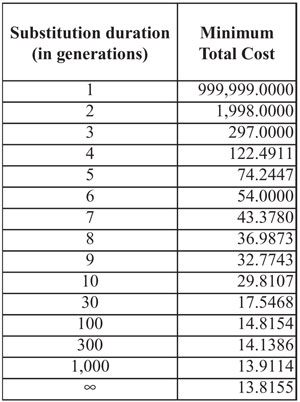
For a substitution of a given duration, a simple proof shows that the lowest total cost is achieved when the cost-per-generation remains constant (see Appendix). Table 2 summarizes this point.

Table 2 is given by the following formula. Let P_S and P_E be the number of copies of the new trait at the start (S) and end (E) of the substitution cycle. Define the ‘substitution growth factor’ K = P_E /P_S . Let N be the number of generations for the substitution. The minimum total cost is given by:

These optimally low costs require the trait to have a constant growth rate throughout all generations. Since nature does not provide this constancy, real cases will always have higher costs. Also, if the new trait decreases even momentarily, then the total cost increases, because some costs will be incurred more than once.

Some theorists believe cost problems can be solved by a non-constant growth rate—such as frequency- or density- dependent fitness, as employed in soft selection.¹¹ But that does not reduce the problem, at least not for single substitutions, as shown above. Rather, constancy is required to minimize the problem, as it allows the lowest possible total cost for a substitution of any given duration.

The total cost is extremely high for fast substitutions, and decreases for slower substitutions. The absolute lowest total cost occurs under conditions never met in nature. It occurs only when the trait increases monotonically, at a constant growth rate, and when that rate is infinitely slow. In that case, equation 4 becomes:

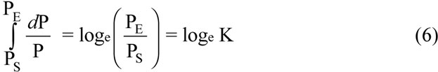
(Note: When N goes to infinity, equation 5 simplifies exactly to equation 6, as expected.)

Table 2. Minimum total cost for increasing a trait by a factor of one million

For a single trait to increase by a given substitution growth factor K, equation 6 gives the minimum total cost under ideal conditions—which are never met in nature. This has also been the most commonly used equation for the total cost of substitution.

Traditional sources of confusion

The cost of substitution depends foremost on the growth rate claimed in a scenario. It is not primarily about the environment, the old-type organisms that are replaced, or their life histories. These had previously been suggested as ways to reduce or eliminate the cost, but they cannot possibly reduce the cost lower than the minimums given above. Their predominant effect is to raise the costs and/or lower the payments, and thereby aggravate cost problems.

Many commentators (e.g. Van Valen,¹² Felsenstein,¹³ Hartl,¹⁴ Merrell⁹ and Grant¹⁵) indicate that according to the cost of substitution, if a population undergoes too many substitutions too rapidly, the cost will be too great and the species will become extinct. That interpretation is faulty. The cost of substitution is not a theory of extinction, and cost, by itself, does not cause extinction. Rather, the cost of substitution supplies a criterion of plausibility, which compels us to reject some scenarios as implausible. Then extinction may, or may not, result for various additional reasons. For example, if a scenario assumes a certain substitution rate is necessary to fend off extinction, then this assumption itself forges the link to extinction, not cost theory. The target of cost theory is the plausibility, or otherwise, of a given scenario.

Some commentators (e.g. Brues¹⁶ and Merrell⁹) suggest ‘the cost of not evolving’ is greater than the cost of evolving. That reckoning uses the word ‘cost’ informally, as though ‘not evolving’ leads to extinction, and extinction has a ‘high cost’. But that interpretation does not correspond to any population genetic definition of cost. Used correctly, ‘the cost of not evolving’—the cost of no substitutions—is zero. Other things being equal, the cost of adaptive evolution is always greater than the cost of not evolving.

The cost of substitution was traditionally taught using the concept of ‘genetic death’. The idea was that a substitution requires the genetic death, or elimination, of the old-type individuals. That created confusion by emphasizing the wrong thing: the death of the old-type, their life history, how they die, and so forth. Fundamentally, the cost of substitution is not about that. It is about the increase—the excess birth—of additional copies of the new-type. The traditional approaches assumed a constant population size, where, in each generation, the actual reduction of the old-type precisely equals the excess births of the new-type. So the concept had some intuitive appeal, and in the simplest cases yielded a correct result. This paper dismisses the concept of genetic death along with the requirement for constant population size.

The above discussion did not mention whether the substituting trait is beneficial, neutral or harmful—because it does not matter. Whenever the trait increases through reproductive means, there is a cost. This contradicts almost all the traditional literature, which holds that neutral substitutions have ‘no cost’ (e.g. Merrell⁹). I clarify the discrepancy by noting that neutral substitutions indeed have a high cost (because they fluctuate up and down, repeatedly incurring additional costs), but their overall substitution rate is not cost-limited.¹⁷ Neutral and slightly harmful mutations individually substitute very slowly, but they have special mechanisms that allow high overall rates of substitution—unlimited by cost—(but instead limited by the mutation rate).

1. Higher payments—There are a few special mechanisms for supplying larger reproductive payments. These mechanisms employ randomness in the payment—a ‘stochastic reproductive excess’ at the level of the individual, plus, in sexual species, also at the level of the gene. [Note: in a sexual species, in each generation, each gene locus experiences a doubling (at fertilization) and halving (at meiosis). From the gene s-eye-view, the ‘doubling’ is a source of reproductive excess, though of a stochastic or random nature. The doubling-and-halving gives an average gene-level reproduction rate of 1.0, but randomly fluctuates above and below that, to provide stochastic reproductive excess. Crossing-over is an additional source. These sources at gene-level are sufficient to pay for substitutions, even if there were no reproductive excess at the level of the individual.] Virtually all of a species’ reproduction is random with respect to a given neutral substitution, and the stochastic component of all that reproduction can be large. This stochastic reproductive excess is what ‘pays for’ genetic drift and the substitutions of neutral and harmful traits. These mechanisms rely on randomness, and are overwhelmingly non-beneficial or harmful in outcome. Within these mechanisms, ‘beneficial evolution’ becomes a moot point.
2. Lower costs—There are also special mechanisms for reducing the average cost of substitution when many mutations occur near each other in time, linked near each other on a chromosome, then they substitute together. In this way ‘many’ are substituted for the cost of one substitution. However, to have much effect, this mechanism requires a super-abundance of the new mutations to be substituted. For example, with unlimited high rates of neutral or harmful mutation, unlimited high rates of these substitutions are achievable—unlimited by cost. Those same mechanisms, however, are not available to beneficial substitutions. Long before those mechanisms can aid beneficial substitutions, the population will be overwhelmed (and destroyed) by harmful mutation. (For example, the desired beneficial mutations would far more often be linked to harmful mutations—so these would travel together, usually to elimination, with no net benefit to the species.) In this case, the cost of eliminating harmful mutation (C_M) would be high—thereby aggravating cost problems. Lastly, the population would likely be in error catastrophe, where harmful mutations would chronically accumulate faster than they could be eliminated. All this happens because harmful mutations vastly outnumber beneficial mutations, in quantity and effect. Long before there is the necessary super-abundance of beneficial mutations, the scenario would suffer severely from high rates of harmful mutation. In such a situation, beneficial evolution becomes a moot point. Evolution must operate within relatively low rates of beneficial mutation, and this precludes this mechanism for reducing the average cost.

In short, while all substitutions have a cost, this fact only limits the beneficial substitution rate. Examples from nature showing rapid rates of neutral or harmful substitution do not contradict cost theory or the cost of substitution, nor do they explain the biological designs that evolution is called on to explain.

Some commentators (e.g. Felsenstein^13,18) have claimed the ‘substitution of favorable mutants in the absence of environmental change does not impose any cost’. That is mistaken. The cost of substitution embodies the unyielding fact that growth requires reproductive excess. The equations given in this paper represent optimal situations, independent of the environment. On average, environmental change can only increase costs and/or decrease payments, thereby intensifying cost problems.

Substitutions when population size fluctuates

Some investigators have argued as follows: suppose the population comprises one million old-type individuals and one new-type individual. If the one million old-type individuals die without heirs, then fixation occurs extremely rapidly, in one generation. Thus, elimination of the old-type (which they equated to ‘the cost of substitution’) places no limitation on the substitution rate. However, that scenario is incomplete, since it does not represent a complete cycle of substitution. It does not represent how evolution happens over the long term. This scenario reduced the population size down to one individual, where countless generations would pass before the next beneficial mutation would occur, allowing the cycle of substitution to begin anew. (For example, a population of one will receive beneficial mutations one million times slower than a population of one million.) This mode of evolution would be exceedingly slow. To speed things up, the scenario can claim the population grows (perhaps returning to its previous size), but that requires reproductive excess—a cost of substitution, as defined above. A speed limit occurs because the population growth rate is limited to the species’ available excess reproduction rate. Once again, the focus on ‘elimination of the old-type’ created confusion by focusing on the wrong thing. The issue is not elimination of the old-type, but rather the growth of the new-type.

This paper takes a broader view of substitution. Under the traditional view, a substitution is defined by changes in allele frequency, and a substitution ‘ends’ at the moment of fixation—thereby excluding any periods where allele frequencies remain constant, and ignoring population growth as irrelevant. That view is inadequate for studying substitution rates over the long term. For this purpose a substitution cycle can be usefully defined as an interval of time beginning with the introduction of a mutation that reaches fixation, then continues after fixation until the introduction of the next mutation to reach fixation. This interval will be at least as long as, and usually longer than, one entire substitution (and may involve substitutions overlapping in time). Under this definition, there is a contiguous set of substitution cycles, with no overlap, or omissions in time. The goal is always to tally the reproductive requirements of the scenario exactly once, with no time periods omitted or counted twice.

The above definition allows calculation of the total cost even when population size fluctuates (which the traditional cost concept did not allow). Such fluctuating scenarios are diverse and awkward to generalize. Their details are an advanced topic, outside this paper. The assumption of constant population size is here taken solely for simplification, so further issues can be clarified.

Haploids, clonal, or self-fertilizing organisms, or maternally inherited cytoplasmic characters

For sake of clarity, the cost concept (defined above) was stated in its simplest, non-genetic form. When applied to specific case studies, the definition can take on the traditional terminology of population genetics—where the substituting ‘trait’ could be a point mutation, insertion, deletion, allele, inversion, duplication, the relative order of genes on a chromosome, or similar. To simplify discussion, the traditional term ‘allele’ will be used as an exemplar for all these.

In a haploid, during a single substitution, let there be P individuals with allele A, and one generation later a scenario claims it increases by ΔP. The cost is given directly by equation 3. Notice this does not depend on the old-type allele, its characteristics, how it dies, or the environment. The cost simply depends on the growth of the substituting allele.

Let N_e be the effective breeding population size. It is typically the number of adults who breed. (Its precise definition is not critical to our calculations, because its impact is solely to measure the population growth or decay. It drops out and has no effect on calculations when it remains constant.) Let the population growth factor When N_e remains constant, G = 1.

The concept of ‘effective producer of progeny’ allows generalization of our notions about reproduction. It allows the conversion of ‘sexual reproducers’ into reproductively equivalent ‘asexual reproducers’. To see how this works, adopt the usual conventions of population genetics. Let the new and old alleles be A and a, with parental frequencies p and q, where p + q = 1. Multiply that equation by N_e to obtain N_e p + N_e q = N_e. The terms of that equation identify the effective producers of the two genotypes. In effect there are N_e p producers of new-type progeny, and N_e q producers of old-type progeny. It is as though all the reproduction of N_e p adults goes to producing genotype-A progeny, and all the reproduction of N_e q adults goes to producing genotype-a progeny. Those figures are exact for asexual species. For sexual species, those figures are average values. In any case, we have subdivided the population’s reproductive capacity into portions responsible for producing each genotype.

A genotype’s effective starting count is the number of effective producers of that genotype. For the substituting allele, that figure is P = N_e p. By definition, the ending count is Then restate equation 3:

Equation 7 is valid under wide conditions, such as erratic fluctuations in both the population size and growth rate of genotype A.

Next, assume a constant population size (G = 1), and utilize the fact that genotype growth is usually specified in terms of selective values. Let genotypes A and a have selective values 1 and 1-s, respectively, where’s > 0.

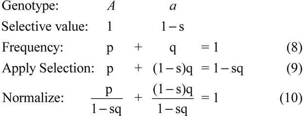
The left-hand term is the new allele frequency , which, by equation 7, gives:

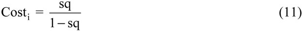
Equation 11 gives the minimum required excess reproduction rate. It is accurate regardless of the environment (changing or unchanging), the selection coefficient (small or large), or the type of selection (soft or hard). For example, in a population of one million adults, where one has the new allele A (therefore, p = 10^-6), suppose s = 1 (which means the substitution occurs in one generation), then Cost_i = 999,999. That reconfirms the first scenario in the above section, cost versus speed.

Genetic death

Equation 11 is identical to Crow’s cost formula, and (under Haldane’s additional assumption of s << 1) it simplifies exactly to Haldane’s formula. This is remarkable because this equation derives from different physical reasoning (though with a similar goal in mind). Haldane reasoned that the population begins with a normalized size of 1 (on the right side of equation 8). After selection, that quantity is reduced by an amount seen at the right side of equation 9 (sq, in this case). Haldane identified this reduction as the genetic deaths divided by the adult population size (so it has units of genetic deaths per adult), and defined it as the ‘cost’. Haldane¹ used this same mathematical method (reflexively, and without physical justification) in all his various case studies. Later, Crow’s formula covered the full range of s-values, but based on the same physical reasoning as Haldane. Crow defined the cost as ‘the ratio of those eliminated (sq), to those not eliminated (1–sq)’. That definition twice uses Haldane’s concept of genetic death.

Their formulas give mathematically correct predictions, but based on dubious physical interpretation. As pointed out by Feller,¹⁹ Moran,²⁰ Hoyle²¹ and Wallace,²² Haldane’s definition of genetic death does not make sense physically, and they give compelling examples of its failure. I here identify the reason. Equations 9 and 10 are separate mathematical steps that represent a single indivisible physical process. In nature, there is no step of applying selection, followed by a separate step of normalizing. Rather, this all happens in one swoop. Haldane’s ‘genetic death’ concept exists only in the middle of these equations (at equation 9). It is a mathematical phantom that does not exist in physical reality. The solution is to jettison his concept of genetic death, and build upon firmer ground.

The physical meaning of a genetic death has been a continual obstacle. Examine the simplest case [a single generation sometime during a single substitution in haploids, with constant population size, and uniform reproduction rate (followed by selection through juvenile death), and s << 1]. In this simplest case, and using the genetic death concept, we can construct a correct argument that limits the substitution rate. But extreme care is required because the logic is indirect and complicated. Firstly, the deaths had to be converted (somewhere, somehow) into a requirement on reproduction rate. Traditionally, this conversion was done implicitly (not explicitly), so it was not well understood.

Secondly, in this simplest case, genetic death was interpreted as a death of old-type individuals caused by the presence of the new allele—or, equivalently, the deaths would not have occurred if the new allele had been absent. So, identifying genetic death seemed to require that the scenario be examined under two circumstances—with and without the substituting allele. But what possible relevance could the second circumstance have? Why would the second circumstance—where substitutions are absent—have any bearing whatever on limiting the substitution rate? This mystery was cause for confusion.

Some researchers interpreted the mystery as follows. If the environment is deteriorating, and the new allele is beneficial relative to the deteriorating environment, then the same deaths would occur even if the new allele had been absent. Likewise, the presence of the new beneficial allele would not increase the deaths. Therefore, the deaths are not caused by the new allele, but are entirely caused by the environmental deterioration. On such a basis, some researchers (e.g. Felsenstein^{13 , 18}) concluded that in a non-deteriorating environment, beneficial substitutions would have zero cost. That faulty conclusion, though still common today, was due to genetic death and the confusion it creates.

In short, even in the simplest cases, many investigators struggled to understand genetic death (of the old allele) and how it could limit the substitution rate (of the new allele). But the situation quickly gets worse. When the scenario moves away from a uniform reproduction rate (and allows selective eliminations due to lowered fertility), then some, or all, of the genetic deaths are virtual, or imaginary (not actual deaths). Haldane said to count these virtual deaths as ‘equivalent’ to real deaths, but he did not explain why. Since these individuals are never even conceived, their physical interpretation is a source of confusion. For example, why would virtual (or imaginary) deaths of the old allele limit the substitution rate of the new allele?

The answer can now be realized. Haldane’s virtual death concept is merely an artificial tabulation device that helps us calculate the correct answer. Tabulate all selective eliminations (even those due to lowered reproduction rate) as though they are actual deaths—that really means all scenarios are calculated as though they have a uniform reproduction rate. (In effect, Haldane was using the cost equivalence principle.) Using that artificial tabulation device (and when the selection coefficient approaches zero), the number of selective deaths of old-type individuals divided by the adult population size (which is Haldane’s cost concept) happens to equal the required excess reproduction rate for the entire population. In other words, there are a certain number of selective deaths of the old-type, and the population is required to produce an excess reproduction rate sufficient to supply those old-type progeny. However, under a uniform reproduction rate, this same rate is also required for producing new-type progeny, and this latter requirement remains unaffected even if the reproduction rate is not uniform (this again uses the cost equivalence principle). In this way, we can translate Haldane’s cost concept (genetic death) into my cost concept, and provide legitimate physical rationale for Haldane’s cost argument.

That rationale, however, is also awkward and convoluted, which has kept Haldane’s argument under a cloud of confusion. Larger selection coefficients add another layer of complication (and confusion). Moreover, when a scenario includes multiple substitutions (overlapping in time), or diploids with non-dominant substitutions, a correct physical interpretation of Haldane’s argument appears intractable. Genetic death quickly becomes a mere mathematical equation, the correct physical interpretation of which is obscure at best.

Nonetheless, many investigators advanced the genetic death concept—and the accompanying confusion fostered various mistaken solutions to Haldane’s Dilemma. They failed to realize that Haldane was not focused on death, but on something else.

Haldane, a consummate mathematician, probably first discovered his cost concept as it lay exposed and beckoning within his math. Haldane’s math accurately predicts something important, but he was grasping at how to explain it. Crow broadened the math somewhat, but based it on the same faulty physical reasoning. Defining cost in terms of reproduction rather than genetic death clarifies the situation by tying the math with physical reality. This is supported by the following fact: in all the various case studies, my substitution cost for a given generation reduces exactly to Crow’s (by assuming a constant population size), and then exactly to Haldane’s (under his additional assumption of s << 1). Yet this cost concept is more general and has a concrete physical interpretation.

Haldane’s¹ paper repeatedly speaks of ‘reproductive capacity’; it was clearly a key focus of his thinking. His paper did not explicitly use the term ‘reproductive excess’, though later commentators, such as Merrell,⁹ understandably attributed that essential concept to him. Crow and Merrell advanced this clearer wording (though still heavily intermingled with the concept of genetic death). Their usage of the term ‘reproductive excess’ further suggests that the cost concept they were grasping for is clarified in this paper. Unfortunately, their proper focus on reproductive excess was largely brushed aside by the rise of a new concept—genetic load.

Genetic load

The substitutional load is defined as the percentage decrease of average fitness within a given generation, caused by the substitution of beneficial mutation. Let w_O be the fitness of the optimal genotype, and let w_A be the average fitness of the population. The substitutional load is (w_O–w_A )/w_A.

In the haploid case, w_O = 1, and w_A = 1–sq, so the load is sq/(1–sq). In other words, the load and cost happen to be equal. (Note: some researchers define load as (w_O–w_A)/w_O = w_O–w_A = sq, which makes load equal to cost so long as s << 1.) A similar equivalence is also found for diploid cases. Kimura popularized this equivalence, and load soon became the predominant way of discussing the cost of substitution. That is unfortunate, because the load concept caused much confusion.

First, cost and load became viewed as identical concepts, when they are different physically. They merely happen to have a weak mathematical equivalence, and then only under special circumstances (such as constant population size, s << 1, etc.). Load obscures the physical processes (especially in diploids), and defocuses the concept of reproduction rate (which is rightly the central focus of cost theory).

Second, substitutional load has a strong counterintuitive flavour. Kimura notes that ‘One popular criticism is that the substitutional load of a more advantageous allele for a less advantageous one cannot be considered a load, since the fitness of the species is thereby increased.’²³ The load argument claims the substitution of a new beneficial mutation into the population temporarily decreases the average fitness of the population, so a beneficial mutation causes a ‘fitness depression’. While that made some sense to mathematicians, its physical interpretation has been a major source of confusion.

Third, load strongly emphasizes the concept of fitness, which creates confusion:

• Fitness values are re-relativized frequently as various mutations enter, exit, or reach fixation, and the timing of which is generally unknown. The continual ‘conveyor-belt’ of re-relativized fitness values creates confusion, much like identifying ‘the tenth man on an escalator’.
• The load calculation depends on w_O , the fitness of the theoretically ‘optimal individual’—whose identity (and fitness) is ever changing. Moreover, in scenarios involving substitutions at many loci, a theoretically optimal individual typically never exists within the population. Load calculations have confusion surrounding the ‘optimal fitness’ (w_O) and how to handle it. (And the current definition of ‘load’ does not clarify it.)
• A given fitness value can be realized with dramatically different tradeoffs between reproduction rate and viability rate. These differences were often viewed as irrelevant, because load focuses so intensely on fitness. This led to indiscriminant use of, and vacillation between, these fitness components, and confusion was the result. (Cost theory focuses on reproduction rate, and thus keeps a clear eye on this distinction.)
• This confusion increases many-fold in situations involving numerous substitutions overlapping in time.

Fourth, load furthered the mistaken idea that neutral substitutions have no cost. This occurred because ‘nearly neutral’ substitutions have ‘very low’ load;²⁴ and neutral substitutions have a load (or fitness depression) of zero, by definition—and load was casually equated with cost.²⁵ Moreover, neutral mutations (and their substitution) cause zero genetic deaths, and this seemed confirmed by the cost equations: since s = 0 for neutrals, their cost (≈ sq) seems to be zero. However, that is a faulty interpretation, because these cost equations are derived using s-values to specify the growth of the allele. When s = 0 there is no growth, and hence no cost—but no substitution either. In effect, it calculates the cost of not substituting a neutral mutation—zero. This again shows a real difference between the load and cost concepts. The erroneous notion that ‘neutral substitutions have no cost’ caused confusion and encouraged various claims that beneficial substitutions likewise have no cost.

Fifth, load is a single value for the entire population (calculated using the entire population’s average fitness, w_A , and optimal fitness, w_O). There is no generally acknowledged method for calculating the load for each genotype, and, even if there were, there is no if-clause to rectify ‘negative loads’ and provide consistent physical meaning suitable for testing scenarios. By contrast, the cost of substitution has a distinct physically meaningful value for each genotype (though usually only the largest costs are calculated for testing a scenario), and these give the reproductive requirements for each genotype. In other words, load theory is a blunt instrument, while cost theory provides finer detail and a more transparent connection to the underlying physical processes.

Cost and load are different lines of physical reasoning. These terms ought to be used more carefully and no longer interchangeably. The cost concept has a direct, clearer physical meaning, while the load concept, in my view, is prone to confusion. In his book Fifty Years of Genetic Load, Bruce Wallace reviews his ‘eventual disenchantment with genetic load theory’.²⁶ An expert user of load arguments, Ewens ‘often sensed a frustration among biologists (including Mayr) … who felt the [prevalent substitutional and segregational load] concepts were misguided but who could not see their way through the mathematical derivations and so find the errors in the load arguments’.²⁷ Load theory brought confusion, and a clarified cost theory can reinvigorate the field.

Continuous-generation models

The discrete-generation model (from equations 3 and 4) can be generalized into a continuous-generation model. At time t, let P(t) and dP(t)/dt be the effective number of individuals who produce type A progeny, and its time rate of change, respectively.

Let T be the effective generation length—this is approximately the parents’ ages when they give each birth, averaged over all births that reach mid-parenthood. T is also equivalent to the time-unit from the corresponding discrete-generation model. This is what links the two models together.

The instantaneous cost per unit time is:

This equation includes the fact that, at any instant, the increase in P is due to the value of P from a time one generation previous. That is, the T-parameter models the time-delay between when progeny are born and when, on average, the next generation of progeny is produced. With this in mind, the analogy with equation 3 is exact. The difference is that equation 3 gives a cost per whole generation, whereas equation 12 gives a cost per infinitesimal time-slice (not per whole generation). Other than that, they both represent the same thing—the required excess reproduction rate.

As before, the total cost merely sums (i.e. integrates) over a substitution cycle.

If the substitution is very slow, compared to the time-delay T, then the total cost will asymptotically approach the classic formula (= log_e K, my equation 6). However, the total cost increases rapidly for faster substitution speeds (as shown in Table 2). This continuous model is directly applicable to haploids, and can be extended to diploids using methods given in the next section.

We can contrast that with Flake and Grant’s continuous-generation haploid model. They define the cost density as ‘the ratio of the instantaneous rate of loss of [the old trait] to the instantaneous population size’.²⁸ Their derivation then arrives at equations identical in form to equations 12 and 13, absent the T-parameter. Their final result then gives a total cost identical to the classic formula (= log_e K, equation 6), independently of substitution speed. This result is inaccurate as no T-parameter was included to model the above-described time-delay between birth and mid-parenthood. Their T is zero (therefore all substitutions are ‘very slow’ compared to their T), and this is why their total cost is independent of substitution speed. This mistake arose because of a focus on genetic death and loss of the old trait—where a ‘time-delay’ would not suggest itself.²⁹ Once again, genetic death was a source of confusion.

Diploids

Since we are interested in required reproduction rates, we must refer to some identifiable reproductive individuals. This paper views the ‘individual’ in the ordinary sense, as a body.³⁰ Therefore, we focus on genotypes, because genotypes correspond to individuals—bodies capable of giving progeny. For example, genotype AA corresponds to a well-defined reproductive body, but allele A does not (as it ambiguously refers to AA or Aa). Alleles substitute, but genotypes are the vehicles for the increases. Therefore, we always calculate the costs of specific genotypes (not alleles). This distinction is invisible for single substitutions in haploids (where the allele and genotype have a one-to-one correspondence), but this distinction is essential in all other cases.

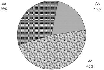
In diploidy, individuals correspond to the three genotypes: AA, Aa and aa. At the start of generation i, let the starting count of breeding adults be denoted as: P_AA + P_Aa + P_aa = N_e . (The ending count of one generation becomes the starting count of the next.) Dividing by N_e gives the starting genotype frequencies, denoted by f_AA + f_Aa + f_aa = 1. The parental allele frequencies are then easily calculated: p = f_AA + ½f_Aa, and q = 1 – p.

Mendelian segregation, in combination with various mating schemes (such as random mating and inbreeding), alter genotype frequencies between parents and progeny, while tending to leave allele frequencies unaffected. By this means, some genotypes can decrease, while others increase. This predictable change is due solely to the passive remixing of alleles at the gene level, and does not require reproductive excess of whole bodies. Therefore, we do not tally it into costs that whole bodies must pay. So we next assess its effect and disallow it from our tally of costs. That is accomplished with the concept of effective producers. I will use random mating to exemplify how all cases are handled.

Random mating produces genotype frequencies given by p² + 2pq + q² = 1. (For other mating schemes, that equation will be different, but the following steps will usually remain the same.) Multiply by the effective breeding size of the population to obtain: N_e p² + N_e 2pq + N_e q² = N_e . That equation gives the effective producers of the three genotypes. (An ‘effective producer’ can be modelled as an abstract asexual adult that, in effect, produces progeny of a given genotype at the same reproduction rate required of its real sexual counterparts.) This parcels the breeding population into three portions, each portion going toward the production of a specific genotype (see figure 3, for example.) It is as though all the reproduction of N_e p² (asexual) adults goes solely toward producing AA genotypes, while all the reproduction of N_e 2pq (asexual) adults goes solely toward producing Aa genotypes, and so forth. That equation shows how the population’s reproductive capacity is redistributed. A genotype’s ‘effective starting count’ is the number of effective producers of that genotype, and is given by the terms of the previous equation, here labelled as P_AA ^* + P_Aa ^* + P_aa ^* = N_e.³¹

As the cycle of one generation completes, call the number of breeding adults the ‘ending count’ (labelled with a prime) as

In generation i, each genotype has a cost, given by equation 3:

Those equations have a straightforward interpretation. Take a case where population size is constant (G = 1), and focus on the substituting genotype AA. Its effective producers have a frequency p² , and this genotype ends the generation at a greater frequency, . That requires a reproduction rate , which is a cost of continuity of 1, plus a cost of substitution of

Within a given generation, the three costs—Cost_AA_i , Cost_Aa_i and Cost_aa_i—do not stack onto each other. They are three separate ‘pipelines’—incurred, and paid, in parallel. The payments that go toward one cannot go toward paying the others.³²

Those three costs are the minimum conceivable cost of substitution incurred by each genotype. Each of those is a ‘mechanical’ limit that cannot go lower, regardless of further details about the selection process. For decreasing genotypes (such as Aa during the second half of the substitution, and aa), this limit is zero. But their cost can, and usually does, go substantially higher. For pure viability selection, all subgroupings of the population have the same reproduction rate (then some unfavoured genotypes are eliminated by premature death); therefore, all genotypes incur the same cost of substitution: Cost_AA_i . On the other hand, for pure reproductive selection, genotypes differ in the rates at which they are produced; therefore, their costs may approach these ‘mechanical’ minimums. In any case, the cost of the substituting genotype—Cost_AA_i—is unaffected by those circumstances, and remains the critical focus for testing the plausibility of a scenario.

It is usually sufficient to focus on the greatest of the three costs, as this cost (and its payment) almost always forms the most stringent test of the scenario: thus:

For a well-behaved substitution, Cost_AA_i always dominates, therefore (by equation 4):

The above method applies under the widest of circumstances. Under the same model assumptions used by Crow and Haldane, the above equations reduce to theirs, including Haldane’s (1957) equations for all his substitution case studies. That includes: (1) haploids, (2) diploids with varying degrees of dominance, (3) inbreeding, and (4) sex-linked loci.³³ For each and every generation, the cost of substitution identified in this paper reduces to the traditional value.

Figure 3. Reproductive capacity is redistributed by Mendelian segregation in diploids. This example shows the percentage of the population’s conceptions that produce progeny of each genotype. In this example, where p = 0.4, only 16% of the conceptions go toward reproducing progeny of genotype AA.

Conclusion

Darwin noted that evolution requires excess reproduction. Cost theory quantifies how much excess is required, and Haldane made a tantalizing initial contribution to the establishment of cost theory.

Haldane¹ was aware his conclusions would ‘probably need drastic revision’. This paper contributes to that revision by:

1. rebuilding the cost concept on foundations more direct, and less confusing, than ‘genetic death’,
2. generalizing the cost concept, thereby eliminating any requirement for: constant population size, small selection coefficients, discrete-generation models, etc.,
3. identifying the compatibility (mathematical, terminological and conceptual) between this clarified cost concept and the traditional thinking,
4. showing the difference between cost and load, and why cost is inherently clearer,
5. eliminating various matters of confusion, such as notions that beneficial substitutions incur ‘no cost’, or ‘pay for themselves’, or ‘cause extinction’,
6. showing that the critical cost of substitution is set by the substituting genotype’s growth rate, and is not reduced by environmental change or the type of selection process (soft or hard).

The treatment given in this paper is fundamental, and will eventually need to be expanded to achieve broadest applicability:

1. scenarios fall into various further categories (depending on the detailed nature of the selection process), each one affecting the cost analysis in distinct ways;
2. multiple substitutions (overlapping in time) introduce additional subtleties into cost calculations;
3. the various other costs (such as the cost of mutation, cost of segregation, and the cost of random loss) must be incorporated, for a complete picture of cost theory and its applications, and these will be addressed in a separate paper.

I share with Haldane¹ and Kimura and Crow³⁴ the belief that quantitative cost arguments ‘should play a part in all future discussions of evolution’. I also agree with George C. Williams that ‘the time has come for renewed discussion and experimental attack on Haldane’s Dilemma’.³⁵

Appendix. Mathematical derivation

The following proof shows that for a single substitution, N generations in duration, the minimum total cost of substitution is achieved when the cost-per-generation remains constant during the substitution. Assume the substituting trait has a unique and consistent physical (cyto-genetic) identity throughout the substitution. Also assume the ending counts for generation i become the starting counts for generation i + 1 (i.e. assume growth of the allele is solely by means of reproductive excess). This proof does not assume constant population size, or anything about the number of old-type traits in the population. For the moment, assume the substitution is in haploids, clonal, or self-fertilizing organisms, or for cases of maternally inherited cytoplasmic characters. Here let an allele exemplify the substituting trait.

At the beginning of generation i, let P_i be the number of copies of the substituting allele in the adult population. (For mathematical simplicity, we here allow P_i to be any positive real number.) For a given substitution, the end-points are fixed at P₀ and P_N (where P₀ < P_N), by definition. In the intervening generations, what values of P_i would minimize the total cost? The proof uses induction; that is, if the theorem is true for N = 2, then it is also true for all larger values of N, because it can be applied repeatedly to each and every pair of adjacent generations. So now we need only prove the theorem for the case of N = 2.

Let the start-and end-points of the two generations be fixed, at P_i and P_i+2 , and we ask, what the mid-value, P_i+1 , should be in order to minimize the total cost of substitution for these two generations alone.

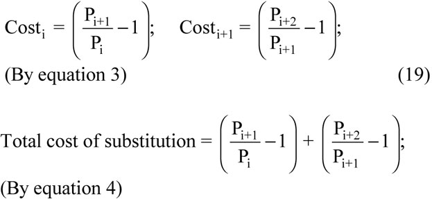
The second derivative (of the total cost with respect to P_i+1) is positive, which means the total cost has a well-defined minimum. To find where the minimum occurs, set the first derivative to zero.

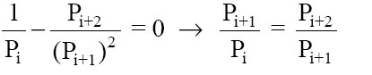
That means (by examination with equation 19), the minimum total cost occurs when P_i+1 has a value that makes the two costs identical. That completes the proof.

Under those same assumptions, dominant substitutions in diploids (with or without inbreeding) can be shown to have a cost of substitution given by equation 19. Therefore, the above proof applies to them as well. The derivation of equation 19 for diploids will be given in a separate paper.

Acknowledgments

This work was supported in part by a grant from Discovery Institute. Thanks also to Dr Paul Nelson.

References

1. Haldane, J.B.S., The cost of natural selection, J. Genet. 55:511–524, 1957. Return to text.
2. Dodson, E.O., Note on the cost of natural selection, Amer. Nat. 96:123–126, 1962. Return to text.
3. Maynard-Smith, J., ‘Haldane’s Dilemma’ and the rate of evolution, Nature 219:1114–1116, 1968. Return to text.
4. Kimura, M., The Neutral Theory of Molecular Evolution, Cambridge University Press, Cambridge, paperback edition, p. 26, 1983. Return to text.
5. Williams, G.C., Natural Selection: Domains, Levels, and Challenges, Oxford University Press, New York, pp. 143–148, 1992. Return to text.
6. Crow, J.F., The cost of evolution and genetic loads; in: Dronamraju, K.R. (Ed.), Haldane and Modern Biology, Johns Hopkins Press, Baltimore, pp. 165–178, 1968. Return to text.
7. Nei, M., Fertility excess necessary for gene substitution in regulated populations, Genetics 68:169–184, 1970. Return to text.
8. ‘Accumulated fertility excess’ was poorly explained and a source of confusion. (E.g. what is the physical meaning of summing the fertility excess across many generations?) Also, Nei noted that he is ‘neglecting mortality due to environmental causes’, thereby neglecting equation 1 and how his concept would relate to it. Also, Nei⁷ defined his concept under a ‘saturated population’ with a constant mean fitness. He did not generalize his concept to handle diploids with dominance, continuous-generation models, large selection coefficients, or non-constant population sizes, and he restricted his discussion to ‘competitive selection at the individual level’. Nei explicitly declined to call his idea a ‘cost’ (such as the ‘cost of natural selection’), and instead coined his more awkward term, above, which prevented the use of convenient terminology: ‘cost’ and ‘payment’. He did not attempt to depose Haldane’s confused cost concept with a clearer one; on the contrary, Nei used his concept merely as a tool for validating Haldane’s cost concept under special circumstances, and concluded that ‘Haldane’s theory of the cost of natural selection appears to be essentially correct even in regulated populations.’ That role was scarcely appreciated at the time, and Nei’s concept, terminology, and conclusion, were largely neglected in the literature. Like Haldane’s concept, it was overwhelmed by confusion, arising from outside and inside his paper. For example, in his debate with Ewens (Ewens, W.J., The substitutional load in a finite population, Amer. Nat. 106:273–282, 1972; and: comments on Nei’s letter on substitutional loads, Amer. Nat. 107:462–463, 1973) over neutral substitutions in diploids, Nei (1973) did not advance his concept. Indeed he could not, because fertility (unlike my reproduction-based concept) cannot be applied at the gene level. That caused a role reversal between Nei and Ewens, ironically, with Nei arguing that neutral mutations have zero substitutional load (or cost), which remains a confusion factor to this day. In this way Nei and Ewens missed an opportunity to resolve what the cost of substitution means. Return to text.
9. Merrell, D.J., Ecological Genetics, University of Minnesota Press, pp.187–193, 1981. Return to text.
10. ReMine, W.J., The Biotic Message, St. Paul Science, Saint Paul, MN, pp. 208–236; 499–507, 1993. Return to text.
11. Wallace, B., Fifty Years of Genetic Load—An Odyssey, Cornell University Press, Ithaca, NY, 1991. Return to text.
12. Van Valen, L., Haldane’s Dilemma, evolutionary rates, and heterosis, Amer. Nat. 47:185–190, 1963. Return to text.
13. Felsenstein, J., On the biological significance of the cost of gene substitution, Amer. Nat. 105:1–11, 1971. Return to text.
14. Hartl, D.L., Principles of Population Genetics, Sinauer Associates Inc., Sunderland, MA, pp. 377–378, 1980. Return to text.
15. Grant, V., The Evolutionary Process, Columbia University Press, New York, p. 166, 1985. Return to text.
16. Brues, A.M., The cost of evolution vs. the cost of not evolving, Evolution 18:379–383, 1964. Return to text.
17. ReMine, ref. 10, pp. 241–245. Return to text.
18. Felsenstein, J., The substitutional load in a finite population, Heredity 28:57–69, 1972. Return to text.
19. Feller, W., On fitness and the cost of natural selection, Genet. Res. 9:1–15, 1967. Return to text.
20. Moran, P.A.P., ‘Haldane’s Dilemma’ and the rate of evolution, Ann. Hum. Genet. 33:245–249, 1970. Return to text.
21. Hoyle, F., Mathematics of Evolution, Acorn Enterprises, Memphis, TN, pp. 111–126; 119–123, 1987. Return to text.
22. Wallace, ref. 11, pp. 76–77. Return to text.
23. Kimura, ref. 4, p 135. Return to text.
24. Kimura, M., Evolutionary rate at the molecular level, Nature 217:624–626, 1968. Return to text.
25. See also Ewens (1972 & 1973) and Nei (1973) for a rare and notable, though wholly indecisive, dialogue on ‘neutral substitutional load’. Return to text.
26. Wallace, ref. 11, p. 139. Return to text.
27. Ewens, W.J., The mathematical foundations of population genetics; in: Singh, R.S. and Krimbas, C.B. (Eds.), Evolutionary Genetics: From Molecules to Morphology, CambridgeUniversity Press, pp. 24–40, 2000. Return to text.
28. Flake, R.H. and Grant, V., An analysis of the cost-of-selection concept, Proc. Nat. Acad. Sci. U.S.A. 71(9):3716–3720, 1974. Return to text.
29. The same argument applies to genetic load, because a ‘time-delay’ would not suggest itself. Return to text.
30. Note: the cost concept can also be applied at other levels, such as the gene level or the species level, where the ‘individual’ is the gene or the species. It may also be applied in other fields, such as the spread of computer viruses, or the spread of neutrons in a nuclear chain reaction—or anywhere reproduction plays a role. In such applications, the cost definition must be rephrased based upon the appropriate reproductive ‘individual’. Return to text.
31. In sexual diploids, the ‘starting count’ and ‘effective starting count’ are no longer identical values, so we here distinguish the latter with an asterisk. Return to text.
32. Note: the mechanisms of reproduction are not physically separated. For example, a genotype-Aa parent participates in producing all three genotypes, however its AA progeny cannot also be Aa or aa progeny. The progeny are destined for one of the three separate ‘pipelines’. Remember we parcelled all the reproduction effectively into three portions that do not overlap or contribute to one another, and that this parcelling can be calculated based on the genetic model and the mating scheme invoked by the scenario. Return to text.
33. Demonstration of this will be dealt with in a separate paper. Return to text.
34. Kimura, M. and Crow, J.F., Natural selection and gene substitution, Genetical Research 13:127–141, 1969. Return to text.
35. Williams, ref. 5, p 148.Return to text.

Anthony P said “Thanks for your … website, it’s really easy to navigate and it is a massive bonus to be able to read back-issues of your magazines … without your ministry I probably wouldn’t be a Christian today. Thank you so much and keep up the good work.” So help us do just that!