
Journal of Creation 22(2):97–104, August 2008
Browse our latest digital issue Subscribe
Molecular limits to natural variation
Darwin’s theory that species originate via the natural selection of natural variation is correct in principle but wrong in numerous aspects of application. Speciation is not the result of an unlimited naturalistic process but of an intelligently designed system of built-in variation that is limited in scope to switching ON and OFF permutations and combinations of the built-in components. Kirschner and Gerhart’s facilitated variation theory provides enormous potential for rearrangement of the built-in regulatory components but it cannot switch ON components that do not exist. When applied to the grass family, facilitated variation theory can account for the diversification of the whole family from a common ancestor—as baraminologists had previously proposed—but this cannot be extended to include all the flowering plants. Vast amounts of rapid differentiation and dispersal must have occurred in the post-Flood era, and facilitated variation theory can explain this. In contrast, because of genome depletion by selection and degradation by mutation, the potential for diversification that we see in species around us today is trivial.
Darwinian evolution

Charles Darwin will always be remembered for turning descriptive biology into a mechanistic science. His famous 1859 book The Origin of Species by Means of Natural Selection, or the Preservation of Favoured Races in the Struggle for Life argued persuasively that species are not immutable creations but have arisen from ancestral species via natural selection of natural variation. Two main points contributed to Darwin’s success:
- he presented a simple, testable, mechanical model that enabled other scientists to engage experimentally with the otherwise overwhelming and bewildering complexity of life;
- unlike others, Darwin approached the subject from many different angles, examined all the objections that had been raised against the theory, and provided many different lines of circumstantial evidence that all pointed in the same direction.
He went wrong in four main areas, however. First, he proposed an entirely naturalistic1 mechanism, but we now know that it must be intelligently designed.2 Second, he extrapolated his mechanism to all forms of life, but we will soon see that this is not possible. Third, he went wrong in proposing that selection worked on every tiny advantageous variation, so it led to the continual ‘improvement of each creature in relation to its … conditions of life.’3 By implication, deleterious variations were eliminated. We now know from population biology that selective advantages only in the order of ≥10% have a reasonable chance of gaining fixation.4 The vast majority of mutations are too insignificant to have any direct influence on reproductive fitness, so they are not eliminated and they accumulate relentlessly like rust in metal machine parts. The machine can continue to function while the rust accumulates, but there is no improvement in the long term, only certain extinction.5
Fourth, he proposed that reproductive success—producing more surviving offspring than competitors—was the primary driving force behind species diversification. If this were true, then highly diversified species in groups like the vertebrates, arthropods and flowering plants would produce more surviving offspring per unit time than simpler forms of life. This is not generally true—quite the opposite. The ratio of microbial offspring numbers per year compared with higher organisms is in the order of billions to one.
Facilitated variation theory
Kirschner and Gerhart’s facilitated variation theory provides a far better explanation of how life works. In a companion article,2 I showed that this requires an intelligent designer to create life with the built-in ability to vary and adapt to changing conditions, otherwise it could not survive. This leads us to the important question of the limits to natural variation.
The limits of natural variation today are extremely narrow, being evident only at the variety and species level. Genesis history requires a far greater capacity for diversification in the ante-diluvian world to be available for rapidly repopulating the Flood-destroyed Earth, and quickly restoring the ecological balances crucial to human habitability. Baraminologists have identified created kinds that range from Tribe (a sub-family category, e.g. Helianthus and its cousins within the daisy family),6 to Order (a super-family category, e.g. cetaceans—the whales and dolphins).7
Theoretical limits to natural variation
Scope for change in core structure
According to facilitated variation theory, the capacity to vary requires:
- functional molecular architecture and machinery,
- a modular regulatory system that maintains cellular function but provides built-in capacity for variation through randomly rearranged circuit connections between machines and switches,
- a signaling network that coordinates everything.
Most variation occurs between generations by rearrangement of ‘Lego-block-like’ regulatory modules. Over this timescale, we can emphatically say that no change at all occurs in the molecular architecture and machinery, because it is physically passed in toto from mother to offspring in the egg cell.
Variation between generations must therefore be limited to the regulatory and signaling systems.
Scope for change in regulatory modules
The law of modules2 says that the basic module of information has to contain functionally integrated primary information plus the necessary meta-information to implement the primary information. This information has to be kept together so that the module retains its functionality.
Genes only operate when they are switched ON. Their default state is to remain OFF. Genes don’t usually work alone, but as part of one or more complexes. Even the several different exons (the protein-coding segments) within a gene can participate in different gene complexes, some being involved with up to 33 other exons on as many as 14 different chromosomes.8 And genes are not just linear segments of DNA, but multiple overlapping structures, with component parts often separated by vast genomic distances.9
Sean Carroll, a leading researcher in developmental biology says, ‘animal bodies [are] built—piece by piece, stripe by stripe, bone by bone—by constellations of switches distributed all over the genome.’10 Evolution, he believes, occurs primarily by adding or deleting switches for particular functions, for this is the only way to change the organism while leaving the gene itself undamaged by mutation so that it can continue to function normally in its many other roles. Carroll considers this concept to be ‘perhaps the most important, most fundamental insight from evolutionary developmental biology.’11
Diversification via Carroll’s proposed mechanism consists of rearranging the signaling circuits that connect up genes, modules and switches, while retaining functionality of both the modules and the organism. Carroll tells us that gene switches are extremely complex, comparable to GPS satellite navigation devices, and easily disabled by mutations, so if switches can be spliced into and out of regulatory circuits, then it must happen via a cell-controlled process of natural genetic engineering (the law of code variation2).
Regulatory areas within gene switches are hotspots for genetic change. An average gene switch will contain several hundred nucleotides, and within this region there will be 6 to 20 or more signature sequences. These signature sequences are similar to credit card PIN numbers—they allow the user to operate the bank account—and they are easy to change. The result of such change is that different signaling molecules will then be able to operate the ‘bank account’ of natural variation.
There are about 500 or so ‘tool-kit proteins’ that are highly conserved across all forms of life and that carry out a wide range of basic life functions. For example, bone morphogenetic protein 5 (BMP5) regulates gastrulation and implantation of the embryo, and the size, shape and number of various organs including ribs, limbs, fingertips, outer ear, inner ear, vertebrae, thyroid cartilage, nasal sinuses, sternum, kneecap, jaw, long bones and stature in humans, and comparable processes in other animals including the beaks of Darwin’s Galápagos finches.
The signature sequences recognized by such tool-kit proteins are usually about 6–9 nucleotides long. A 6-nucleotide sequence can have 46 = 4096 different combinations of the nucleotides T, A, G and C, and a 9-nucleotide sequence can have 49 = 262,144 different combinations. But there are 6 to 20 or more signature sequences that can be recognized by the 500 different tool-kit proteins, which gives somewhere between 5006 (~1016) to 50020 (~1054) different possible combinations.
An obvious limitation to change in regulatory circuits is that switches can only switch ON functions that already exist. It is easy to switch OFF an existing function, but it is impossible to switch ON a function that does not exist.
Two examples of regulatory variation are given in figure 1. The hair dryer and the vacuum duster both use similar materials—motorized fan, plastic housing, power circuit and switch. In one, the control circuit is wired up to blow air; in the other, the circuit is reversed, and the machine sucks air. A biological example is the axolotl, a salamander that has retained its juvenile gills into adulthood. This can happen if there is an iodine deficiency in the diet, or if a mutation disables thyroxin production. By adding thyroxin, the axolotl will develop into a normal salamander. Both these switch-and-circuit rearrangements seem to be simple changes, but they are possible only because complex mechanisms of operation already exist within the system.
Scope for change in signaling networks
While there is enormous potential for variation built-in to the circuitry that connects up regulatory modules, it is signals that trigger the switches and their functional modules. What scope is there for diversification in signal networks?
Signal networks are compartmented. They operate as a cascade within each compartment—one signal triggers other signals, which trigger other signals etc. Each compartment cooperates with its adjacent compartments so that the unity and functionality of the organism is maintained, but they do not influence activities beyond their local neighbourhood.

The two examples I used to illustrate this point in the companion article ‘How Life Works’2 were the propagation of plants from cell culture, and the regeneration of double-headed and double-tailed planarian flatworms. In both these cases, a single signal molecule triggered a dramatic developmental cascade (shoot/root growth in the former, and head/tail growth in the latter) that was completely independent of, but cooperative with, the other half of the whole organism.
Some signals are hard-wired into the cell, while others are soft-wired. An example of a hard-wired signal occurs within the apoptosis cascade for dismantling cells and recycling their parts. In a normal cell, apoptosis is extensively integrated with a wide range of functional systems and can be triggered by a variety of causes through a complex signaling network. However, in human blood platelets the system is isolated from its normal whole-cell environment and we can see it operating in a much simpler form.
A complex of two proteins, Bcl-xL and Bak, performs the function of a molecular switch. When Bcl-xL breaks down, Bak triggers cell-death.12 In a normal whole cell, homeostasis maintains the balance between Bcl-xL and Bak, but platelets are formed by the shedding of fragments from blood cells and there are no nuclei in them. Once the platelets are isolated from homeostatic control, Bcl-xL breaks down faster than Bak, so the complex provides a molecular clock that determines platelet life span—usually about a week. No signal is sent or received in this hard-wired system, so there is no room for diversification.
Hard-wired signaling networks are probably a major component of stasis. We can visualize them by using a domino cascade model, illustrated in figure 2. In this case, embryogenesis is symbolized as a series of events in the main circle, which trigger other peripheral cascades as they proceed. Each cascade continues until it meets a STOP signal, at which point the whole circuit is shut down. A similar thing happens in individual cells when they differentiate. Embryonic stem cells have the potential to become any cell in the body, but once the cascade is traversed, all options but one are shut down.
In contrast, a soft-wired system sends actual signal molecules, raising the possibility of adaptive change—e.g. sending a different signal molecule. A recent study of red blood cells investigated cell fate decision making—whether to proliferate, to kill themselves or to call for help. This decision lies at the very heart of homeostasis because it determines the robustness and stability of the organism in the face of change and challenge.

The researchers discovered that they did not need to know the detailed structure of the decision-making system, just a knowledge of its network of signaling interactions was sufficient to identify which components were the most important.13 This finding was confirmed in another study in which a wide range of perturbations were applied to white blood cells and the effect upon the cell fate decision was examined. The decision came not from any particular target of perturbation, but as an integrated response from many different nodes of interaction in the signaling network. The authors suggested that computations were carried out within each node of the signaling network and the combination of all these computations determined what the level of response should be from any particular perturbation.14
Does this indicate a potential for adaptive change? Or does it suggest a system that is designed to resist change?
The primary role of the signaling system is to coordinate everything towards the goal of survival. Life can survive only by maintaining a balance between contradictory objectives. On the one hand, it has to achieve remarkable results as accurately as possible—e.g. plants turning sunlight into food without the high energies involved killing the cell. On the other hand, it has to do it in an error-tolerant and constantly variable manner to maintain its adaptive potential and its robustness and stability.
The solution to this dilemma is error minimization. All possible routes will involve risks of error, but the optimal solution will minimize those risks. A computer simulation study of regulatory networks found that using an error minimization strategy leads to the formation of control motifs (gene switching patterns) that are widely found in very different kinds of organisms and metabolic settings.15 When applied to the ‘noise’ in yeast gene expression that results from the ON/OFF nature of signaling, it was found to also be the case in real life. Genes that were essential to survival exhibited the lowest expression-noise levels when compared with genes that were not directly essential. The author concluded that ‘there has probably been widespread selection to minimize noise in [essential] gene expression.’ But there is a down side—noise minimization probably limits adaptability.16

Since the goal of signal coordination is survival, I suspect that the large, interconnected signaling networks in all forms of life contribute more to stasis than to change.
Practical limits to natural variation
It is impossible to describe the full range of natural variation across all life forms in a journal article, so I will focus just on variation within the grass family (Poaceae), and between it and other families of flowering plants (Angiosperms).
The grass family comprises about 10,000 species in about 700 genera. Is it possible that maize, lawn grass and bamboo all arose from a common ancestor? Baraminologists believe so.17
Grass morphology
The easiest way for us to conceptualize the extent of natural variation is through illustrations of morphological variations. We need to keep in mind that much more than morphological variation is involved in speciation, but it can serve as a convenient surrogate for our present purpose. The basic structure of a generalized grass flower (spikelet) is illustrated in figure 3.

A common variation on the standard structure is the development of an awn upon the apex of the lemma (or glume) in figure 1C. This transformation is fairly straightforward. The apex of the lemma is extended into a long straight awn, then a regulatory change causes the edges to grow faster than the centre, which causes the base part of the awn to spiral around into a twisted column, leaving a straight or curved bristle at the top.
Grasses generally have a multitude of spikelets, arranged into a terminal structure called the inflorescence, as shown in figure 4.
Species-level variation in the Australian salt grass Puccinellia
Salt grasses of the genus Puccinellia are distributed worldwide, from the Antarctic to the Arctic, and they occur right across southern Australasia (Australia and New Zealand) in marine salt marshes, around the edges of inland salt lakes and on salinised pasture lands. They have a quite generalized grass morphology, with no special adaptations for dispersal, as many other grasses do, so they may represent a typical primordial grass.
The most widespread species, found right across Australasia, is Puccinellia stricta. When Edgar18 described the New Zealand species in 1996 she noted some differences between Australian and New Zealand populations of P. stricta and suggested that further detailed study was warranted. I was fortunately able to undertake that study,19 with results that are quite typical of many widespread plant genera. My study focused on the genus in Western Australia (WA), where three native species were identified—P. stricta, P. vassica and P. longior. An ordination and classification of specimens based on their morphological characteristics is shown in figure 5.

The plot shows that all three species are well separated from one another, with members of each species being more closely similar to members of their own species than to other species.
I then needed to know how our specimens of Puccinellia stricta compared to specimens of the same species from right across Australasia. Loan specimens were obtained from other herbaria and the same analysis was carried out as for the WA specimens. A very different plot resulted, as shown in figure 6.
In this case, a new species was clearly separated out from the rest, while the remainder spread broadly right across the ordination space. The group labeled perlaxa (occurring only in southeast Australia) had previously been identified as a subspecies of stricta, but from this analysis it was clear that it warranted species status, so we named it Puccinellia perlaxa.
The big picture of the native Australasian species of Puccinellia that emerged from this study was of a single widespread species, P. stricta, that varied in a continuous manner right across the whole region, and then localized species with restricted distributions that could generally be explained in terms of local ecological and/or geographical factors.
Historically, therefore, it is most likely that the widespread species was the progenitor of the all the other species. It has retained at least some of its capacity for variation, and certainly a greater capacity (wider dispersion in the ordination space) than any of the other species that I studied.
Morphological variation in Australian Puccinellia


Australian Puccinellia species vary most markedly in their panicle structure, a few of which are illustrated in figure 7.
Puccinellias have multiple florets per spikelet, ranging from 3 or 4 up to 10 or more. One feature that varies significantly in spikelet structure is the length of the upper glume, illustrated in figure 8.
The palea also varies significantly, particularly in the extent of hairs on the margins, as shown in figure 9.
Genus-level variations in Tribe Paniceae
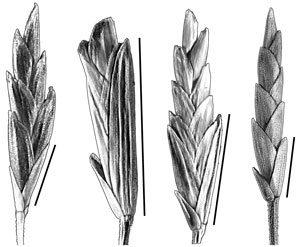
The grass family is divided up into Tribes of genera that (ideally) reflect their common ancestry. The largest Tribe is Paniceae, and Häfliger and Scholz have suggested that the spikelet variations within this Tribe follow a fairly simple pattern of retrogression from the original Paniceae spikelet,20 as illustrated in figure 10.
Sub-family variation within Poaceae
Argentinian researchers Vegetti and Anton have shown that if we begin with a panicle as the primordial grass inflorescence, then every other generic form can be derived simply by adding, subtracting, shortening or lengthening the components of the panicle.21 I will take just three types of transformations that represent different sub-family groups within Poaceae—wheat, maize and silkyhead lemon grass.
Wheat
The hypothesized transformation of a panicle structure into the reduced seedhead of a wheat plant via the Vegetti-Anton theory is illustrated in figure 11.
Maize

Transformation of a panicle into the compact seedhead of maize is more complex, but still conceivable, as illustrated in figure 12. The primordial panicle could have been divided by the panicle branches being switched OFF in the mid-section, and leaf modules being turned ON. A leaf within the inflorescence is called a ‘spathe’ leaf. Apical dominance is a common mechanism in all plants for repressing growth below the apex until conditions are appropriate. This normally controls the proliferation of fertile seeds within grass spikelets. It represses female organ development more strongly than the male parts, so in many grasses the apical florets within a spikelet will be either male or sterile, and only the lower florets (those furthest away from the dominating apex) will produce fertile seed. This mechanism is already in place to suppress female organ development in the top branches of the maize plant, making them all male. But the lower branches of the inflorescence are now far distant from the apex, so apical dominance is eliminated and the female organs grow uninhibitedly, perhaps out-competing the male organs and suppressing them altogether. Leaf and bract growth in the lower parts is stimulated and they cover the female spike entirely. This causes the female florets to lengthen their pollen receptors so that they can reach the open air and receive wind-dispersed pollen, making the silky tassel at the end of a corn-cob.
Silkyhead lemon grass

Transformation of the panicle into silkyhead lemon grass (Cymbopogon obtectus) can be hypothesized by reducing the pedicel of alternate spikelets so that they occur in pairs—one pedicellate, the other sessile. The pedicellate spikelet retains apical dominance and is sterile or male, and the sessile spikelet is fully fertile, but it also develops an awn on its lemma (see figure 3). The paired branching structures occur also in pairs, and a leaf growth module is switched ON within the developing inflorescence to produce a spathe leaf surrounding each pair of branched structures. Hairs are normally present in many parts of the inflorescence, and are usually short, but in Cymbopogon obtectus, the hairs are abundant and long, producing a fluffy white ‘silkyhead’ at flowering time, as illustrated in figure 13.
Origin of the angiosperms
Within the grass family, diversification from a common ancestor seems to be fairly straightforward, and could have occurred via numerous rearrangements of parts that were already present in the primordial grass ancestor. But can we continue this process back to a common ancestor with daisies, orchids and all other flowering plants?
A recent review of the subject was entitled ‘After a dozen years of progress the origin of angiosperms is still a great mystery.’22 The ‘progress’ referred to was the enormous effort put into DNA sequence comparisons, in the belief that it would give us the ‘true’ story of life’s origin and history. While such comparisons have proved of great value in sorting out species and genus relationships, the results for family relationships and origin of the angiosperms has often been confusing and/or contradictory—thus the remaining ‘mystery’.
Recent discoveries of fossil flowers show that angiosperms were already well diversified when they first appeared in the fossil record. The ‘anthophyte theory’ of origin, the dominant concept of the 1980s and 1990s, has been eclipsed by new information. Gnetales (e.g. Ephedra, from which we get ephedrine), previously thought to be closest to the angiosperms, are now most closely related to pine trees. To fill the void, new theories of flower origins have had to be developed, and ‘Identification of fossils with morphologies that convincingly place them close to angiosperms could still revolutionize understanding of angiosperm origins.’22
Conclusions
Theoretically, the greatest scope for natural variation appears to lie in the almost infinite possible permutations of the Kirschner–Gerhart ‘Lego-block’ regulatory module combinations, and these could rapidly produce the enormous diversification implied by Genesis history. In contrast, there is no scope at all for change in the machinery of life from one generation to the next because it is passed on in toto from the mother in the egg cell. Signaling networks appear to be limited in their scope for diversification, particularly those that are hard-wired (designed into the system) into compartments and cascades that have symmetry and functional constraints. The elaborately interconnected signaling networks are very robust in the face of perturbation, and provide a crucial component of stasis. There is some potential for variation in the signaling molecules that are sent, but error minimization limits its functional scope.
From a practical point of view, diversification of the whole grass family from a common ancestor is conceptually feasible via switching ON and OFF the original component structures within a primordial grass. It is not possible to switch ON components that don’t exist, however, so this mechanism cannot be extrapolated to include a common ancestor between grasses and other angiosperms such as daisies and orchids.
Flowering plants display an enormous amount of differentiation and dispersal (between 250,000 and 400,000 species in 400 to 500 families worldwide) and appear only in the upper levels of the fossil record. Most of this diversification appears therefore to have happened rapidly, possibly in the post-Flood era. A possible reason for this is that the flowering plants were originally planted in the Garden of Eden and radiated worldwide mainly after the Flood.23
This is not Darwinian evolution. It is intelligently designed, built-in potential for variation in the face of anticipated environmental challenge and change. The word ‘evolution’ is still useful in describing processes of historical diversification, but its Darwinian component is now only a minor feature. In contrast to Darwin’s proposed slow development of variation, the evidence supports a vast amount of rapid differentiation in the past, degenerating into only trivial variations today—a far better fit to Kirschner–Gerhart theory and Genesis history.
Acknowledgments
I am grateful for the comments from three referees and numerous colleagues, which have helped to improve this article.
Recommended Resources
References
- Darwin mentioned a Creator on the last page of The Origin, but later regretted it, acknowledging it was only a concession to public opinion. Private letter from C. Darwin to J. D. Hooker, Down, Friday night (17 April 1863), <darwin-online.org.uk/content/frameset?viewtype=side&itemID=F1452.3&pageseq=30>, 23 May 2008. Return to text.
- Williams, A., How life works, Journal of Creation 22(2):85–91, 2008. Return to text.
- Darwin, C.R., The origin of species by means of natural selection, or the preservation of favoured races in the struggle for life, John Murray, London, 6th ed., Summary of Chapter IV, 1872. Return to text.
- Haldane, J.B.S., The cost of natural selection, Journal of Genetics 55:511–524, 1957; Maynard Smith, J., The Theory of Evolution, Penguin Books, Harmondsworth, UK, p. 239, 1958. Return to text.
- Williams, A., Mutations: evolution’s engine becomes evolution’s end!, Journal of Creation 22(2):60–66, 2008. Return to text.
- Cavanaugh, D.P. and Wood, T.C., A baraminological analysis of the Tribe Heliantheae sensu lato (ASTERACEAE) using Analysis of Pattern (ANOPA), Occasional Papers of the Baraminology Study Group, No. 1, June 17, 2002. Return to text.
- Wood, T.C., Wise, K.P., Sanders, R. and Doran, N., A refined baramin concept, Occasional Papers of the Baraminology Study Group No.3, July 25, 2003. Return to text.
- Kapranov, P., Willingham, A.T. and Gingeras, T.R., Genome-wide transcription and the implications for genomic organization, Nature Reviews Genetics 8:413–423, 2007. Return to text.
- Birney, E. et. al., Identification and analysis of functional elements in 1% of the human genome by the ENCODE pilot project, Nature 447:799–816, 2007. Return to text.
- Carroll, S.B., Endless Forms Most Beautiful: The new science of Evo Devo, Norton, New York, p. 111, 2005. Return to text.
- Carroll, S.B., Evolution at two levels: on genes and form, PLoS Biology 3(7):1159–1166, 2005; p. 1162. Return to text.
- Qi, B. and Hardwick, J.M., A Bcl-xL timer sets platelet life span, Cell 128(6):1035–1036, 2007. Return to text.
- Grimbs, S., Selbig, J., Bulik, S., Holzhütter, H.-G. and Steuer, R., The stability and robustness of metabolic states: identifying stabilizing sites in metabolic networks, Molecular Systems Biology 3:146, 2007. Return to text.
- Kumar, D., Srikanth, R., Ahlfors, H., Lahesmaa, R. and Rao, K.V.S., Capturing cell-fate decisions from the molecular signatures of a receptor-dependent signaling response, Molecular Systems Biology 3:150, 2007. Return to text.
- Shinar, G., Dekel, E., Tlusty, T. and Alon, U., Rules for biological regulation based on error minimization, PNAS 103(11):3999–4004, 2006. Return to text.
- Lehner, B., Selection to minimise noise in living systems and its implications for the evolution of gene expression, Molecular Systems Biology 4:170, 2008. Return to text.
- Wood, T.C., A baraminology tutorial with examples from the grasses (Poaceae), Journal of Creation 16(1):15–25, 2002. Return to text.
- Edgar, E., Puccinellia Parl. (Gramineae: Poeae) in New Zealand, New Zealand J. Bot. 34(1):17–32, 1996. Return to text.
- Williams, A.R., Puccinellia (Poaceae) in Western Australia, Nuytsia 16(2):435–467, 2007. Return to text.
- Häfliger, E. and Scholz, H., Grass Weeds 1: Weeds of the Subfamily Panicoideae, CIBA-GEIGY, Basel, Switzerland, pp. xiii–xiv, 1980. Return to text.
- Vegetti, C. and Anton, A.M., The Grass Inflorescence; in: Grasses: Systematics and Evolution, Proceedings of the Third International Symposium on Grass Systematics and Evolution, Jacobs, S.W.L. and Everett, J. (Eds.), CSIRO Publishing, Melbourne, pp. 29–31, 2000. Return to text.
- Frohlich, M.W. and Chase, M.W., After a dozen years of progress the origin of angiosperms is still a great mystery, Nature 450:1184–1189, 2007. Return to text.
- Genesis 2:9—only angiosperms would appear to fit the description ‘pleasing to the eye and good for food’. Return to text.


Readers’ comments
Comments are automatically closed 14 days after publication.