This article is from
Journal of Creation 33(1):110–118, April 2019

Browse our latest digital issue Subscribe

Patriarchal drive in the early post-Flood population

by Robert W. Carter

The book of Genesis gives us a clear picture of human history. Specifically, Genesis 9:18–19 claims that all people alive today descend from Noah’s family. In the Table of Nations (Genesis 10), we see a genealogical description of multiple people groups who lived within a few hundred miles of the author. And in Genesis 11 we have a chronogenealogy that gives us not just the names but also the lifespans and the age of each Patriarch when the next generation is born.¹ This is invaluable information, and we can use it to shape our expectations of the size and mutation burden of the modern world population.^2,3

Yet, mutation rate studies have not yielded the ‘true’ mutation rate, even though it is of critical interest. Modern sequencing projects (e.g. 1,000 Genomes) use high-throughput techniques that create vast amounts of short sequence reads that then need to be run through sophisticated algorithms to produce an alignment. With a high enough coverage, sequencing errors can be averaged out. But very often low coverage data is instead compared to a standard (e.g. the already-assembled human genome). This provides great information for large-scale genomic features like inversions and large indels, but, due to the inherent error rate of the DNA polymerases used to generate the short reads, it is impossible to infer the real mutation rate from the data. Some authors have gone so far as to use a ‘fixed’ date in secular archaeology (e.g. the peopling of the Americas) and then call it a ‘sanity check’ for any mutation rate calibrations.⁴

For these and other reasons, the Y chromosome mutation rate has had various estimates.^5,6 Helgason et al.⁶ reported a rate of 8.71×10^–10 per nucleotide site, per person, per year for the Y chromosomes of a selection of Icelandic males. This translates to 3.14 × 10^–8 per site, per person, per generation, using a 36-year generation time.⁷ Given a sequenced portion of the Y chromosome of approximately 30 million bases, this amounts to just under 1 mutation (0.942) per person per generation, in modern Icelandic males. This is probably not a good proxy for the mutation rate of all men, across the world, throughout all human history, but it is all we have to go on at present. In biblical history there have been only a few hundred generations. At this assumed mutation rate, it might be possible to explain the history of the majority of extant Y chromosome lineages (figure 1). However, specific lineages (e.g. some rare lineages found in Africa) have accumulated enough mutations to make them difficult to explain with the modern mutation rate alone, so further analysis is required. Denisovans and Neandertals (see Discussion), which are expected to be as different in their Y chromosomes as they are in the rest of their genomes, are a separate case that will require additional modelling and brainstorming. They could be the result of an extreme form of what is being discussed in this paper, or the data could be spurious (less likely over time as more ancient genomes are sequenced), or some not-yet-discovered factor could be at play.

Can we estimate the Y chromosome mutation rate in long-lived ancient men? During human development, spermatogonia undergo more cellular division then eggs. But eggs also remain in an undivided state until fertilization several decades later. In men, however, the germ cells start dividing rapidly at puberty and continue to divide until the man’s death. This simple difference between sperm and egg production produces different mutation patterns from the maternal and paternal sides.⁸ It also means more mutations are expected to come from the father than the mother.⁹ But this rate should also scale with paternal age. This is of singular importance for biblical models of human history, where great ages of the early generations are inherent.

The paternal age effect is well known.^10,11 Not only do sperm display increased genomic decay with age on the gross architectural level,¹² but sequencing reveals that the mutation burden increases with the age of the father. The effect also appears non-linear.¹³ Yet, we have zero opportunity to test it in men with ‘biblical’ ages of several centuries, meaning we can only speculate about the mutational burden given to us from Noah and his children and grandchildren. From studies of modern men, we have learned that differences can arise in different spermatogonial lineages within a single man, meaning one parent can produce greatly differing offspring,¹⁴ depending on which spermatogonial lineage contributed to each child. In fact, some spermatogonial lineages can ‘take over’ in an almost cancer-like or selection-like scenario.¹⁵ This might have an analog in the mutator strain hypothesis and the non-clocklike mutation accumulation at essentially every scale in the Y chromosome phylogenetic tree.^16,17 It also means that Shem, Ham, and Japheth could have received very dissimilar Y chromosomes from Noah, or that one of the brothers could have been quite different from the other two. There is no reason to expect every male to receive the same number of mutations, but there is every reason to expect centuries-old men to pass on many times more mutations than the modern average.

Yet, nearly all mutations that occur today are lost to random drift.¹⁸ The probability of any man giving rise to a brand-new major branch of the Y chromosome family tree is exceedingly remote. But the potential ‘impact’ of any new mutation is the inverse of the population size. That is, in an exponentially growing population, the percentage of individuals expected to carry an allele at time t + 1 is about the same as the percentage carrying it at time t. This is of utmost importance when discussing the post-Flood world. The probability of a new lineage forming is greater when the population is small, but this is also the time when the Patriarchs are alive and fathering children.

Carter, Lee, and Sanford¹⁴ introduced the term ‘patriarchal drive’ in their study of modern human Y chromosomes and mitochondrial DNA. This is defined as the genetic effects of long-lived people in a small population who become parents at great ages. But what effect might they have? That would depend on the immediate post-Flood mutation rate and how it scales with the father’s age, the rate of early population growth, and how evenly distributed the children were within the population. In other words, if a ruling class developed early, they could easily have suppressed reproductive output among the lower classes. We see evidence for this even late in history. For example, about one in five men from Northern Ireland (including this author) share a Y chromosome lineage that is associated with the Uí Néill clan, which may or may not trace their ancestry to a 6^th century Irish chieftain named Niall of the Nine Hostages.¹⁹ Another example is that of Genghis Khan, who lived in the 13^th century but is ancestor of perhaps 0.5% of the modern world population.²⁰ Over time, even a slightly favourable reproductive advantage among one group would have been profound, effectively reducing the male population size to much less than the real size. In fact, it might be assumed that the longest-lived men in the population, those with the fewest number of generations from Noah, would more often become princes and rulers, and thus have an advantage over the majority of other males.

We also know that there are statistically significant differences in branch lengths among multiple Y chromosome groups that had a clear common ancestor.¹⁴ Thus, throughout human history the ‘molecular clock’ has not ticked at the same rate across time and geography. How much of the discrepancy could be due to paternal drive? Some, but certainly not all. Figure 1 shows multiple individuals that have longer branch lengths (i.e. more mutations) than closely related contemporaries (going counterclockwise, examples can be seen in groups C, G, I, O, T, M, and K). These differences have arisen in recent history, well after the Patriarchs were deceased. And yet, the results of the current study predict that long branches can form quickly and early. Putting these two things together tells us that the molecular clock simply cannot be trusted.

But there are numerous unknowns in this discussion. In fact, we know nothing about most of the important variables. Thus, we need a flexible model if we are going to test the effects of patriarchal drive in the early post-Flood world. Yet, several biblical population models have already been developed.^21-23 These have been shown to be both useful and realistic. The only thing required would be to add a model of mutation accumulation and track the ancestry of each individual. There is no need to force the model to generate evidence of patriarchal drive. If the effect is real, it should appear naturally, once the proper factors are being measured, within the models already in existence.

Methods

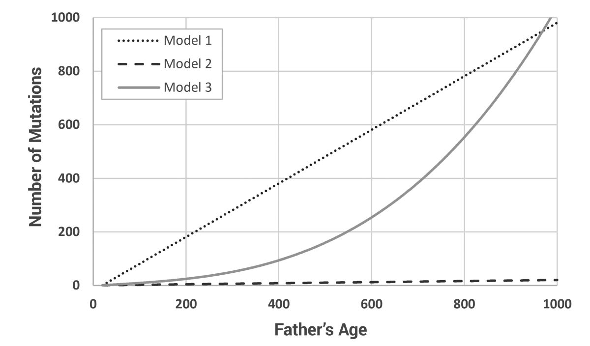
Working from the models of Carter and Hardy²¹ and Carter and Powell,² a new model, written in Perl, was developed that allowed for the tracking of mutations in a post-Flood-like population. Other than the ages of paternity and total lifespan of a few individuals, almost nothing is known about the life history parameters of the early post-Flood population. Thus, three contrasting mutation models were developed to bracket the most likely possibilities (figure 2). All models assume that at least one mutation will be passed from father to son each generation. Model 1 is a simple linear model where the number of Y chromosome mutations equals the father’s age, less 20 years to allow for a prepubescent period of dormancy [y = 1 + age – 20]. This creates unrealistically high mutation rates at young ages. Model 2 is another linear model using the factor of ‘2 extra mutations per extra year of father’s paternity’ from Kong et al.,²⁴ but also assumes that only 1% of all mutations will occur on the Y chromosome [y = 1 + (age – 20) x 0.02]. This fixes the problem with Model 1 at young ages, but almost certainly under-represents the mutation rate at high ages. Model 3 is a polynomial model developed as a best guess of the expected mutation curve [y = 1 + (age – 20)/10 + ((age – 20)/100)³]. This produces normal values in the known age ranges (paternal ages of 20 through 50 produce from one to four Y chromosome mutations in the son) and exponentially increasing mutation counts in the ‘biblical’ age categories.

Starting parameters

The model started with three reproducing couples. Each founding individual was already 100 years old and lived for another 500 years, approximating the age of Shem at the Flood and his total lifespan.²⁵ The starting number of mutations depended on the mutation model and the simplifying assumption that Noah was 500 when the three sons were born. Basic parameters are given in table 1.

An age of maturity started the mutation clock. People could get married after this. Children could be born the next year. Minimum spacing between children was set to 15 years. This sounds extreme, but population growth had to be slowed to better simulate real-world expectations (i.e. the world population did not reach multiple billions of people until modern times), even though this meant each couple had fewer children. To reduce ‘cohort’ effects where all people of a certain age are having children simultaneously, the probability of a child being born after the minimum spacing was exceeded was set to ⅓ per year.

Lifespan reduction

Each subsequent generation lived 85% as long as the previous generation (average of mother’s and father’s maximum lifespan × 0.85), with a minimum lifespan of 80 years. This reduction rate was chosen to reflect the rate of lifespan reduction after the Flood: from Shem to Joseph, each subsequent generation had an average lifespan of 88% (+/– 23% SD) of the previous one. There is a high variance to these numbers, with three generations living longer than the generation prior to it. Attempts were made to develop a lifespan reduction model based on year of birth, cumulative age of paternity at birth, etc., but the 85% approximation was chosen because it is both simple and intuitive. Even though modern people often live longer than 80 years, and many ancient people did as well, men tend to not have many children at high ages, so a maximum lifespan of 80 seemed like a reasonable compromise. The age of menopause for females was set at 80% of total lifespan, for simplicity. One final assumption of the model was that menopausal women did not get remarried after the death of their husband, but widowers could get remarried and continue to have children up to the year of their death.

Mutation accumulation

Mutations were assigned to each child when it was born based on the age of the father only and according to the formulas for the chosen mutation model (figure 2).

Generational penalties

To mimic an assumed reproductive advantage for men fewer generations removed from Noah, a generational penalty was assigned to each birth. A list of children to be born each year was generated. For each child, a random number was assigned based on the paternal generation count of the father from Noah—e.g. ‘rand (paternal_generations)’. This provided a 15-digit floating-point number between 0 and the generation count. Men with fewer generations had a higher chance of obtaining a smaller number than men of later generations. After sorting, a preset percentage of the children were allowed to be born. A 50% cut-off generally drove the population extinct. The model runs reported in this paper allowed for 75% of all slated births to go through. Allowing for 100% removed the generational penalty entirely.

Birth replacement

Since this project was performed on a personal laptop, computer processing needs had to be kept to a minimum. The CPU clock rate (2.7 GHz) was not a critical requirement, as long as the models did not take many hours to finish, but available RAM (12.0 GB) was. Thus, the most important factor was the number of individuals being tracked. Carter and Hardy (2015) and Carter and Powell (2016) showed that populations of 5,000 or more individuals were a good approximation of any larger population size. A maximum population size was assigned for each model run, equal to 10,000 individuals for the results presented in this paper. When the population reached this size, a random individual was chosen to be overwritten each time a baby was born. High replacement levels increased the likelihood that Patriarchs could be lost, but this was held in check by the rapidly reducing lifespans (natural deaths made room for babies) and slower population growth rates (figure 3). The presence of replacement added a random component and meant there was no need to follow a life history table for the calculation of random deaths (cf. Carter and Hardy 2015). A model that did not end prematurely due to population extinction always had some replacement. If birth spacing was too large (e.g. a minimum of 20 years between births) the population would begin to decline after the long-lived Patriarchs died off. Thus, the goal was to always have a net excess of births in order to model a robust, growing population.

Artificial chromosomes

Since the paternity of each male in the model was known, it was possible to create artificial chromosomes that tracked the entire population history. For each model run, an array with n rows and 100,000 columns was created and all values were initialized to zero. A position counter incremented for each new mutation in the population. If at any time the total number of mutations exceeded the width of the array, an extra 1,000 bits were added to each row and initialized to zero. When a boy was born, his father’s row was copied to his. He then received X new mutations, so X bits were set to 1, starting at the last position + 1. In this way, every column in the array contained a unique mutation inherited from a specific ancestor. At the end of the run, the array was translated into a pseudoDNA sequence (each 0 was translated into an A and each 1 was translated into a G), and the data were saved in FASTA format. The three founding male ancestors were assigned a tag, depending on the number of mutations called for by the mutation model, either 000000…, 111111…, or 010101… This translated into AAAAAA…, GGGGGG…, or AGAGAG… and appeared at the beginning of any chromosome in the model when it finished running. But because many mutations drifted out of the population (i.e. some men had no living descendants) any column with no variation was skipped. The FASTA file was imported into the phylogenetics modelling software MEGA (version 7.0.26),²⁶ from which several standard phylogenetic trees could be created. The neighbour-joining method was chosen for this paper due to its simplicity (sequences are grouped into closest pairs, then pairs of pairs are grouped, etc.) and the fact that it makes no evolutionary assumptions within internal branches (as in the case of several other tree building methods). However, alternate tree-building algorithms produced essentially the same results (data not shown).

Results

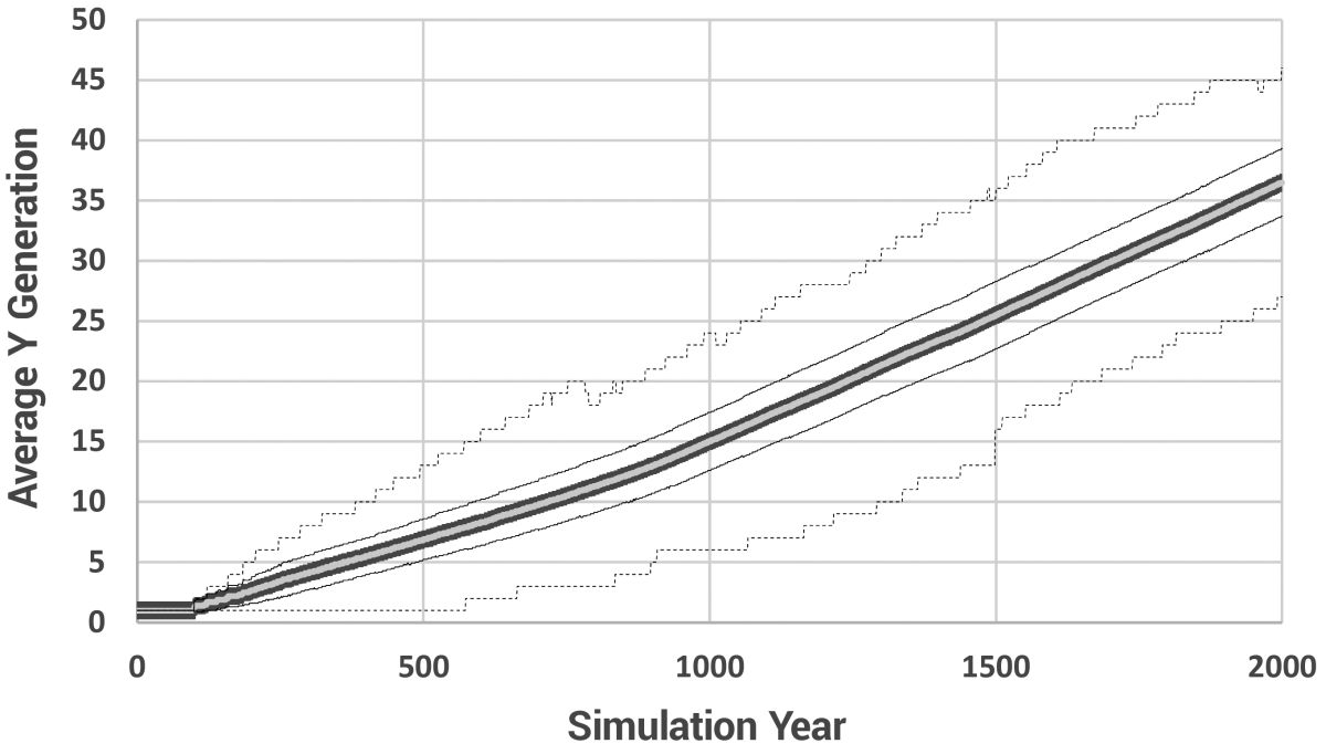
Figures 3 to 10 were generated from the Model 3 results, but since all three mutation models had identical population parameters, they produced essentially identical results for these basic statistics. In fact, subsequent model runs were highly reproducible.

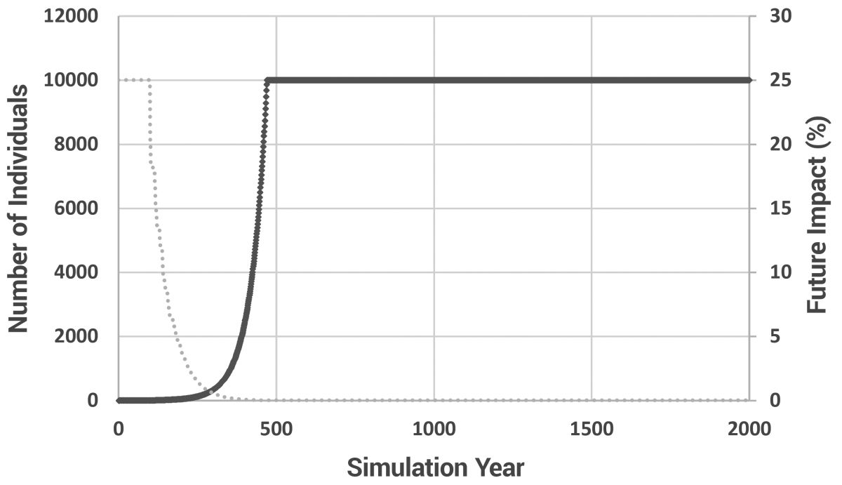
Due to the nature of exponential growth, even with an age of maturity of 20 years and a 15-year minimum spacing between children, the population still grew rapidly, taking approximately 470 years to reach the pre-determined maximum of 10,000 individuals (figure 3). Increasing the maximum population size did little (it took only 575 years to reach 100,000 individuals). In this model, there is no ‘soft landing’. When the maximum population size is reached, newly born children simply replace existing individuals. This ‘replacement’ model is valid as long as only a small fraction of individuals are replaced each year. Too much replacement and the effects of Patriarchal drive would be masked by the removal of too many older people from the population. Since we know the Patriarchs lived to great ages, obviously they were not ‘replaced’ prior to their recorded age at death. Thus, keeping replacement to a minimum was a necessary compromise between the requirements of the biblical model and available computer processing power.

The number of births, marriages, deaths due to old age, and losses due to replacement in the model over time are given in figure 4. As the average lifespan drops, more people die each year. This creates more space for new children and necessitates fewer replacements of living individuals over time. The average (+/– 1 SD), minimum, and maximum lifespans per model year are shown in figure 5. The timing was chosen as a compromise, essentially delaying the time it took to reach maximum population size for as long as possible.

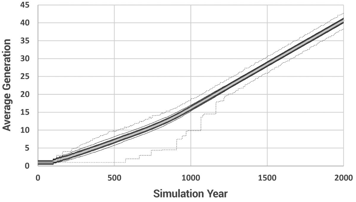
The gradual reduction in lifespan is shown in figure 5. The average number of generations and the average number of paternal generations are shown in figures 6 and 7, respectively, and a histogram showing the range of paternal generations at various model years is given in figure 8.

Figures 9–11 show the most significant results of this project. Figure 9 displays the average number of new mutations entering the population per model year. The total range is much greater than shown. One individual received 210 mutations in year 558 alone, but since the population was so large by then, he had little effect on the average. The stochasticity is caused by the nature of sampling in small populations. In other words, when the population is very small, the average is strongly determined by whether or not a Patriarch has a child that year. But note that the average number of mutations directly translates to average branch length on the phylogenetic tree. These results indicate a strong potential for faster-than-modern mutation accumulation rates in the early post-Flood population. They also tell us to expect variable branch lengths, even among branches rising contemporaneously.

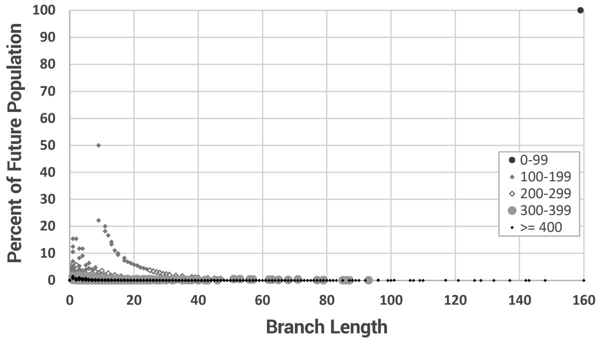
This is more clearly shown in figure 10, where the branch length for every new individual is shown. The data are grouped into irregular time intervals and the point styles adjusted for maximum distinction. The initial generation (Noah to Shem, Ham, and Japheth), would have created three massive new branches 160 mutations long (using mutation model 3). Since the model starts with only three men, 100% of the men carry branches that long at year zero. After that, long branches were continually added, but at extremely low frequencies after year 300. This shows us that long branches can form instantaneously early in the biblical model and then be carried to a significant proportion of the modern population.

However, these results are strongly dependent on the mutation model (figure 11). In fact, since we know nothing about the mutation rates among the long-lived, early post-Flood Patriarchs, we can only draw cautious conclusions.

Figure 12 displays a phylogenetic tree from a small model population. We can see early and deep branching, the result of strong genetic drift, and multiple features that appear similar to figure 1, such as the ‘tufts’ of closely related individuals at the end of long, straight branches. This is a very interesting line of research, but as of now the ability to do this is more of a ‘proof of concept’. It is memory-intensive and generating a tree for 5,000 men that tracks 100,000 or more mutations is near the limit of most desktop computers. Much more work needs to be done.

Discussion

Mutation accumulation is a real-world problem that must be cracked if we are to develop a working biblical model of human history. Multiple factors contribute to it, but most of the parameters are unknown. The best we can do, then, is to model different possibilities and see how they comport to expectations. Here, patriarchal drive has been shown to be a real possibility and should be incorporated into any basic model of biblical genetics developed in the future. Very old men fathering children in a small but growing population should have a profound effect on the early branching patterns in the Y chromosome family tree. Long branches can and should have formed early in human history, independently of any molecular clock. Yet, the results depend strongly on the mutation model, the rate of population growth, and multiple demographic trends we know nearly nothing about.

The three dissimilar models were chosen for two main reasons. First, they bracket real-world expectations. Second, they show that much more work needs to be done. There is much we simply do not know. However, the results presented here naturally derive from already established population models. No ‘tweaking’ of any parameters was required, other than the development of the dissimilar mutation models. One might be concerned that Model 3 underestimates Model 1 (the uppermost linear model in figure 1) at the maximum model age (600 years). However, the real problem is that Model 1 is not realistic at normal, modern maximum ages (i.e. <100 years). Since we cannot know how many mutations were passed down by the biblical Patriarchs, all we can do is create a range of estimates and hope to improve these estimates with further experimentation.

DNA polymerases make mistakes and mistakes are expected to accumulate over the life of an individual, as the number of cell divisions since fertilization increases. The mutator strain hypothesis,¹⁴ however, is an additional factor that may come into play, but it only partially overlaps the expectations of patriarchal drive. If a small population contains individuals with a defective DNA repair system, for example, the entire population might accumulate many more mutations than expected over a certain time span. Sperm lack DNA repair mechanisms, but DNA repair is active in spermatogonia.²⁷ Thus, damage to Y chromosomes through defects in DNA repair systems can occur at any life stage. Can this explain the discordant lineages found among the click-speaking people groups of Africa (e.g. the Pygmies of the Central African forest and the Khoi-San bushmen of Southern Africa)? It might well explain the presence of haplogroup A00 in Cameroon. When geneticists discovered the Y chromosome of a descendant of Albert Perry (an African slave who lived in South Carolina, US) in a commercial genealogy database, they were surprised. He had a brand-new branch, never seen before. Searching revealed that very few men in Central Africa carried related lineages which were dubbed A00, the “basal-most” branch among all living men.²⁸ But there is a major problem with this: extremely rare lines should drift out of a population quickly. How could the ‘oldest’ line have maintained itself in a rare state for approximately 200,000 years?²⁹ Mathematically, this makes no sense. Rupe and Sanford showed that nearly all new mutations quickly drift out of a population.¹⁶ The more rare a variant, the more likely it is to be lost due to random chance. All new mutations, by definition, start off in a single individual and are thus maximally rare. In standard population genetics, the probability of any variant becoming fixed is equal to 1/n. The probability of a variant becoming lost is the converse of this, 1 – 1/n. Extremely rare lineages, therefore, are not expected to persist for any length of time, yet the A00 line is both extremely rare and extremely old? Instead, it is more likely this is a new line that has simply experienced an elevated mutation rate in recent times. This would produce a discordant branch more quickly.

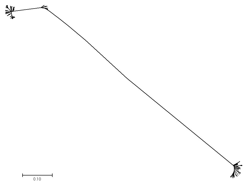
There are other important factors not considered in this paper, but they all should play a part in the global story of mankind. Selective sweeps were not discussed, neither were population surges,¹⁵ but these two factors will dramatically affect what we see. Consider figure 1. There are multiple ‘tufts’ sitting at the end of long branches (e.g. the two E1 and R1 clusters). The beginning of each tuft represents a historical male who had a surprisingly large number of male descendants. Rare but important, or simply lucky, males have produced most of the extant lines. All other lines are extinct. Thus, population surges are a strong driver of the final shape of the tree. Drift and selection are often difficult to tell apart, but in figure 12 strong drift is evident. Nearly all early side branches have gone extinct, leading to two main ‘tufts’ on long, slender branches. Almost all of the remaining individuals are closely related to other individuals and a great mutational distance separated the groups from each other.

Neandertals and Denisovans are also not yet part of this model. There are several reasons for this. First, there is but one partial Neandertal Y chromosome available to date.³⁰ Also, its quality is questionable. Consider figure S11 in the much-discussed paper on ancient Canaanite DNA by Haber et al.³¹ Since mutations accumulate in all lineages over time, modern people should have more mutations than ancient people. The most ancient samples should be on the shortest branches. Yet the opposite is true here. This casts a suspicious light on all ancient DNA studies. For example, the long branches we see for the Neandertals and Denisovans might be artifactual. Second, we need to learn a lot more about inbreeding effects in small populations (Neandertals and Denisovans are the most inbred populations we have ever seen).³² Third, we need to formulate a theory of how they drifted from the root of mankind so quickly.

In the end, we expect a chaotic early history of man. That is, even if the events are fixed in history, it will be very difficult to predict the exact pattern that should result from the starting conditions. The combination of rapid early population growth, patriarchal drive, fragmentation of the population after Babel with the subsequent long-term isolation of some groups and extreme inbreeding in some, population surges and collapses, and selective sweeps (either naturally or through war and conquest) creates a recipe for exactly the type of tree we see, even if the specific tree cannot be predicted. In figure 1 there are deep branches that separate all major lineages, yet there are only a handful of these lineages. The paucity of major lineages indicates that we came from a small population that expanded rapidly. The distance between the lineages suggests patriarchal drive was in effect during the early years of that expansion. How much of an effect this had depends on many factors that have yet to be fleshed out, but patriarchal drive should be considered an important part of the discussion.

References and notes

- Sarfati, J., Biblical chronogenealogies, J. Creation 17(3):14–18, 2003. Return to text.
- Carter, R.W. and Powell, M., The genetic effects of the population bottleneck associated with the Genesis Flood, J. Creation 30(2):102–111, 2016. Return to text.
- Carter, R., Effective population sizes and loss of diversity during the Flood bottleneck, J. Creation 32(2):124–127, 2018. Return to text.
- Carter, R.W., Lee, S.S., and Sanford, J.C., An overview of the independent histories of the human Y chromosome and the human mitochondrial chromosome; in: Whitmore, J.H. (Ed.), Proceedings of the Eighth International Conference on Creationism, Creation Science Fellowship, Pittsburgh, PA, pp. 133–151, 2018; creationicc.org/abstract.php?pk=364. Return to text.
- Xue, Y. et al., Human Y chromosome base-substitution mutation rate measured by direct sequencing in a deep-rooting pedigree, Current Biology 19(17):1453–1457, 2009. Return to text.
- Helgason, A. et al., The Y-chromosome point mutation rate in humans, Nature Genetics 47:453–457, 2015. Return to text.
- Skov, L. et al., Analysis of 62 hybrid assembled human Y chromosomes exposes rapid structural changes and high rates of gene conversion, PLoS Genetics 13(8):e1006834, 2017. Return to text.
- Jónsson, H. et al., Parental influence on human germline de novo mutations in 1,548 trios from Iceland, Nature 549:519–522, 2017. Return to text.
- Crow, J.F., Age and sex effects on human mutation rates: an old problem with new complexities, J. Radiation Research 47:Suppl. B75–B82, 2006. Return to text.
- Walter, C.A. et al., Mutation frequency declines during spermatogenesis in young mice but increases in old mice, PNAS 95:10015–10019, 1998. Return to text.
- Francioli, L.C. et al., Genome-wide patterns and properties of de novo mutations in humans, Nature Genetics 47(7):822–826, 2015. Return to text.
- Kaarouch, I. et al., Paternal age: negative impact on sperm genome decays and IVF outcomes after 40 years, Mol Reprod Dev 85(3):271–280, 2018. Return to text.
- Yoon, S-.R. et al., The ups and downs of mutation frequencies during aging can account for the Apert syndrome paternal age effect, PLoS Genet 5(7):e1000558, 2009. Return to text.
- Choi, S-.K., Yoon, S.-R., Calabrese, P., and Arnheim, N., A germ-line-selective advantage rather than an increased mutation rate can explain some unexpectedly common human disease mutations, PNAS 105(29):10143–10148, 2008. Return to text.
- Goreily, A. and Wilkie, A.O.M., Paternal age effect mutations and selfish spermatogonial selection: causes and consequences for human disease, American J. Human Genetics 90:175–200, 2012. Return to text.
- Carter, R.W., Lee, S., and Sanford, J.C., An overview of the independent histories of the human Y-chromosome and the human mitochondrial chromosome; in: Whitmore, J.H. (Ed.), Proceedings of the Eighth International Conference on Creationism, Creation Science Fellowship, Pittsburgh, PA, pp. 133–151, 2018; creationicc.org/abstract.php?pk=363. Return to text.
- Sanford, J. et al., Adam and Eve, designed diversity, and allele frequencies; in: Whitmore, J.H. (Ed.), Proceedings of the Eighth International Conference on Creationism, Creation Science Fellowship, Pittsburgh, PA, pp. 200–216, 2018; creationicc.org/abstract.php?pk=363. Return to text.
- Rupe, C.L. and Sanford, J.C., Using numerical simulation to better understand fixation rates, and establishment of a new principle: Haldane’s Ratchet; in: Horstemeyer, M. (Ed.), Proceedings of the Seventh International Conference on Creationism, Creation Science Fellowship, Pittsburgh, PA, 2013. Return to text.
- Moore, L.T., McEvoy, B., Cape, E., Simms, K., and Bradley, D.G., A Y-chromosome signature of hegemony in Gaelic Ireland, American J. Human Genetics 78:334–338, 2006; See also irishtimes.com/news/science/the-genetic-imprint-of-niall-of-the-nine-hostages-1.1771373. Return to text.
- Zerjal, T. et al., The genetic legacy of the Mongols, American J. Human Genetics 72:717–721, 2003. Return to text.
- Carter, R. and Hardy, C., Modelling biblical human population growth, J. Creation 29(1):72–79, 2015; creation.com/population-growth. Return to text.
- Hössjer, O., Gauger, A., and Reeves, C., Genetic modeling of human history part 1: comparison of common descent and unique origin approaches, Bio-Complexity 2016(3):1–15, 2016. Return to text.
- Hössjer, O., Gauger, A., and Reeves, C., Genetic modeling of human history part 2: a unique origin algorithm, Bio-Complexity 2016(4):1–36, 2016. Return to text.
- Kong, A. et al., Rate of de novo mutations, father’s age, and disease risk, Nature 488(7412):471–475, 2012. Return to text.
- Hardy, C. and Carter, R., The biblical minimum and maximum age of the earth, J. Creation 28(2):89–96, 2014; creation.com/biblical-age-of-the-earth. Return to text.
- Tamura, K., Stecher, G., Peterson, D., Filipski, A., and Kumar, S., MEGA6: molecular evolutionary genetics analysis version 6.0, Molecular Biology and Evolution 30:2725–2729, 2013. Return to text.
- Gunes, S., Al-Sadaan, M., and Agarwal, A., Spermatogenesis, DNA damage and DNA repair mechanisms in male infertility, Reprod Biomed Online 31(3):309–319, 2015. Return to text.
- Mendez, F.L. et al., An African American paternal lineage adds an extremely ancient root to the human Y chromosome phylogenetic tree, American J. Human Genetics 92: 454–459, 2013. Return to text.
- Elhaik, E. et al., The ‘extremely ancient’ chromosome that isn’t: a forensic bioinformatic investigation of Albert Perry’s X-degenerate portion of the Y chromosome, European J. Human Genetics 22:1111–1116, 2014. Return to text.
- Mendez, F.L. et al., The divergence of Neandertal and modern human Y chromosomes, American J. Human Genetics 98:728–734, 2016. Return to text.
- Haber, M. et al., Continuity and admixture in the last five millennia of Levantine history from ancient Canaanite and present-day Lebanese genome sequences, American J. Human Genetics 101(2):274–282, 2017. Return to text.
- Reich, D. et al., Genetic history of an archaic hominin group from Denisova Cave in Siberia, Nature 468:1053–1060, 2010. Return to text.
Readers’ comments
Comments are automatically closed 14 days after publication.