

Journal of Creation 24(2):105–107, August 2010
Browse our latest digital issue Subscribe
Where are we in the universe?
Fourier analysis of galaxy number counts N(z) calculated for both the large galaxy surveys, SDSS and 2dF GRS, indicates that galaxies have preferred periodic redshifts. There are two ways to interpret this data: 1) that the effect is purely in redshift space and therefore results of some observer bias and/or the universe underwent past oscillations in its expansion rate, or 2) that it is a real space effect and due to the physical location of millions of galaxies on concentric shells with regular spacings. These explanations can be tested and preliminary analysis favours the latter. If this turns out to be true, it means our galaxy is located about 125 million light-years from the centre of the largest super-structure of galaxies ever observed.
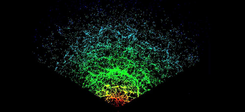
Millions of sources in the cosmos have been located by robotic telescopes and various data recorded for them. From that, maps have been created that show how the galaxies are distributed in the sky around our galaxy. Figure 1 shows one such map generated with many tens of thousands of galaxies. At the apex we find our galaxy, but the scale of this map is huge. This is from one such survey, the Sloan Digital Sky Survey (SDSS), and another is the 2 degree Field Galaxy Redshift Survey (2dF GRS).
In a recent paper,2 a colleague and I showed from the Fourier analyses on galaxy number counts N(z) calculated for both SDSS and 2dF GRS, that galaxies have preferred periodic redshifts. Discrete Fourier Transforms were calculated from N(z), the histograms determined by binning (counting) the observed redshifts of the survey galaxies between z – δz/2 and z + δz/2 as a function of redshift z, where generally δz = 10-3 was used. Data for 427,513 galaxies from the SDSS Fifth Data Release were obtained where the data are primarily sampled from within about -10 to 70 degrees Declination from the celestial equator. Also, data for 221,414 galaxies were obtained from the 2dF GRS where the data are confined to within 2 degrees Declination balanced between the Northern and Southern hemispheres.
The analysis found significant redshift spacings of Δz = 0.0102, 0.0246, and 0.0448 in the SDSS, with significance at a level of at least 4σ,3 and strong agreement with the same analysis from 2dF GRS. If one then applies the Hubble law,4 that is, assumes that the Hubble law,

applies to these relatively low redshift galaxies (z < 0.35) without assuming any cosmology, then the conclusion one gets is that the galaxies preferentially tend to be located on concentric shells with periodic real space intervals. These were determined from Eq. (1) by replacing z with Δz, resulting in regular real space radial distance intervals Δr. And by combining the results from both surveys we get Δr = 31.7 ±1.8 h-1 Mpc, 73.4 ± 5.8 h-1 Mpc and 127 ± 21 h-1 Mpc, where the Hubble constant H0 = 100 kms−1 Mpc−1 and the parameter h = H0 /100, as used in standard cosmology.
In the usual analysis, in standard cosmology, the spatial two-point or autocorrelation function is used to define the excess probability, compared to that expected for a random distribution, of finding a pair of galaxies at a given separation. This involves the assumption of the Cosmological Principle.5 As a result the power spectrum P(k) is derived from the two-point correlation function.6 The power spectrum is predicted by theories for the formation of large scale structure in the universe and compared with that measured, or, more precisely, calculated from the available data.
The power spectrum P(k) is used to look for mass density fluctuations on various scales over cosmological time. There it is assumed that looking back in redshift space is looking back over cosmological time and, in the light of the Cosmological Principle, any density fluctuations are simply evidence of the scale of clustering at some past epoch (z), since there is no special or preferred frame to view the universe from.
In deriving P(k), a windowing function (usually a Gaussian) is applied to reduce the noise seen in the density fluctuations as a function of k or 1/Δz. But it also has the effect of smoothing out the ‘signal’ we are looking for contained in the ‘peaks’ at small redshift intervals (1/Δz). After applying this method, without the Gaussian windowing function, we did still find significant redshift space (actually k-space) periodicity in both data sets at redshifts intervals consistent with the first two listed above, i.e. at Δz = 0.0102 and 0.0246. However a Discrete Fourier Transform (FT) of the unsmoothed N(z) data is much more sensitive to finding redshift space periodicity at smaller values of Δz. And the third significant redshift periodicity, where Δr =127 ± 21 h-1 Mpc, seen with the FT method, is the same result discovered by Broadhurst et al. (1990)7 from a pencil-beam survey of field galaxies. The latter is generally interpreted as the scale of galaxy clustering in the universe.
Also, we applied straight pair counting. Another way to determine if galaxies are separated by a periodic redshift interval is to build histograms by binning the number of pairs (Npairs) of galaxies that have the same separation (Δz) in redshift space, then looking for over abundance peaks in the Npairs histograms. Since redshifts are measured radially from the observer at the centre of the distribution this method detects redshift space separation with respect to that symmetry. As it turned out, it was not so sensitive but did still detect the first two listed above, i.e. at Δz = 0.0102 and 0.0246.
Finally we did a correlation analysis between the two surveys. We compared N(z) from each by artificially shifting the redshift of the ith bin (determined between zi – δz/2 and zi + δz/2) in one survey and recalculating the correlation function R2 each step. See ref. 2 for details. There is a significant spatial region of the 2dF GRS that has overlap with the SDSS and so we would expect R2 for the unshifted bins to show significant correlation. What we found was interesting. We found a periodicity in the R2 correlation function with a period Δz ≈ 0.027. This is again the main visible-to-the-eye redshift periodicity in figure 1. Now these results can be interpreted as either evidence for a real space structure with our galaxy cosmologically near its centre, or as a redshift space effect where the universe has undergone oscillations in its expansion rate over past epochs. The latter is what Hirano et al. (2008)8 advocated and we referred to in ref. 2.
Either the effect is totally due to the expansion of the universe, and therefore only a redshift space effect, because redshift is one dimensional, or it results from real space structure. Since we are only able to sample the radial component of the redshift, assuming it results from the galaxies moving away from us, then it would only appear that the galaxies are arranged in rings (or shells in 3D space) due to the fact that in the past the universe’s rate of expansion oscillated. If this were the case then it should look like all galaxies are racing away from the centre and that these rings are centred exactly on the observer, never off-centre from the observer, not even by a small amount.9
The subtlety here is that one is implicitly assuming that the distribution of galaxies in the universe must be essentially random on the very large scale with only the cosmic web of filaments and voids, an assumption from the Cosmological Principle. Hence anything else you see must be due to some effect other than real space structure.
“What really interests me is whether God had any choice in the creation of the world”—Albert Einstein10
However if the effect is a real space effect, it means that the galaxies are physically situated in concentric shells, which, in an expanding universe, are moving away from us at the centre. This interpretation also suggests that, at a minimum, the local universe we see around us has a special place, a centre, and we are there, or nearby. This idea is at odds with the Cosmological Principle, which remember has its origin in the notion that there is no Creator, no design and no purpose in the universe. Therefore, the idea that we may be living at or near the centre of the universe is abhorrent to all those who hold to atheistic and/or non-biblical worldviews.
It is not so easy to determine the real space structure of the universe because we have no independent measure of distance in the universe. So when astronomers look at a map, like in figure 1, they really are looking at a map of redshifts and directions in the sky from where the light has come. Then to get the distance to the source galaxy they have to assume the Hubble law.
But there may be a way to distinguish between the two possibilities. As I mentioned, if the centre of the large scale structure of galaxies around us coincides with our galaxy then it would suggest that it is purely a redshift effect and not indicative of real space, though even that would still be impossible to prove because we have no independent measure of distance. But if the centre of concentric shells of galaxies coincides at some other point in space then that indicates a real space structure and not solely a redshift space effect.
In a second paper11 I found that a real space superstructure, possibly involving millions of galaxies, was favoured, with galaxies preferring to lie on periodically spaced concentric shells centred on a location about 26.86 h-1 Mpc from here. Certainly, to date, this has not been ruled out. However, I made the assumption that for small redshifts it was valid to assume we are looking at spatial distribution of the galaxies in their redshifts. Then I implemented an algorithm to artificially shift the centre in real space, recalculate what all the redshifts would be if observed from that new central point, determine N(z) and recalculate the FT from the new N(z). I then compared the magnitude of the second Fourier peak (redshift space interval) to determine where the true physical centre should be. This is where the Fourier peak amplitude is maximized.
I found that the centre of the concentric shells with Δz ≈ 0.027, which are most prominently seen in figure 1, does not coincide with our galaxy’s position in space but that the centre is about 26.86 h-1 Mpc or about 125 million light-years (assuming h = 0.72) from here. That is still a relatively small distance on the scale of the very large scale of the structure analysed—billions of light-years in extent.
Near centre of massive super-structure of millions of galaxies
The evidence is in favour of this effect being due to real space structure because the spherical shells of periodic redshift are not centered on our galaxy. If it was a systematic effect due to observer bias then we would expect that the centre of the shells would coincide with the observer. Though this is still not conclusive, and more analysis is needed, we have evidence for a supermassive real space structure, possibly involving millions of galaxies, with our Milky Way located somewhere near but not actually at its centre.
We are in a special place after all, both spiritually at the centre of God’s attention and also maybe physically somewhere near the centre of the largest galactic structure ever observed in the universe. We are here not by random chance but because God created the earth to be inhabited and He wanted to show us His glory.
“For the invisible things of him from the creation of the world are clearly seen, being understood by the things that are made, even his eternal power and Godhead; so that they are without excuse” (Romans 1:20).
And they are without excuse.
References
- For a more detailed and complete map, where luminosity is represented by colour, see: www.sdss.org/news/releases/galaxy_zoom.jpg. Return to text.
- Hartnett, J.G. and Hirano, K., Galaxy redshift abundance periodicity from Fourier analysis of number counts N(z) using SDSS and 2dF GRS galaxy surveys, Astrophysics and Space Science 318(1, 2):13–24, 2008; preprint available at: arxiv.org/abs/0711.4885. Return to text.
- I.e. Four standard deviations. Return to text.
- Hubble law: v = H0 r, where v is the velocity of the expansion of the universe, as determined by the redshift of the galaxies in it. Here redshift z = v/c for small redshifts, where c is the speed of light in a vacuum. The distance to the galaxy is represented by r, and H0 is the Hubble constant, which has been very difficult to determine but nowadays lies somewhere between 55 and 80 km/s/Mpc. Return to text.
- It essentially assumes that the galaxies in the universe are uniformly yet randomly distributed throughout the cosmos on some very large scale. Therefore all observers at all locations in the universe at the same epoch should see the same distribution of galaxies. There are no favoured places. Richard Feynman succinctly describes the problem of the Cosmological Principle:
“ … I suspect that the assumption of uniformity of the universe reflects a prejudice born of a sequence of overthrows of geocentric ideas … It would be embarrassing to find, after stating that we live in an ordinary planet about an ordinary star in an ordinary galaxy, that our place in the universe is extraordinary … To avoid embarrassment we cling to the hypothesis of uniformity.” Feynman, R.P., Morinigo, F.B. and Wagner, W.G., Feynman lectures on gravitation, Penguin Books, London, p. 166, 1999. Return to text. - The power spectrum is essentially the square of the Fourier frequencies in k-space but calculated with a windowing function. Here k=1/Δz is the inverse of the redshift interval. Return to text.
- Broadhurst, T.J., Ellis, R.S., Koo, D.C. and Szalay, A.S., Large-scale distribution of galaxies at the Galactic poles, Nature 343:726, 1990. Return to text.
- Hirano, K., Kawabata, K. and Komiya, Z., Spatial periodicity of galaxy number counts, CMB anisotropy, and SNIa Hubble diagram based on the universe accompanied by a non-minimally coupled scalar field, Astrophys. Space Sci. 315:53, 2008. Return to text.
- This situation would also be indistinguishable from real space structure exactly centred on our galaxy. Return to text.
- Einstein made this remark to Ernst Straus, his assistant from about 1950–1953 at the Institute for Advanced Study at Princeton (Holton, G., Einstein’s third paradise, Daedalus, Fall 2003, pp. 26–34; p. 30, www.aip.org/history/einstein/essay-Einsteins-Third-Paradise.pdf, accessed 7 May 2010). Return to text.
- Hartnett, J.G., Fourier analysis of the large scale spatial distribution of galaxies in the universe; in: Proceedings of the 2nd Crisis in Cosmology Conference, Potter, F. (Ed.), Port Angeles, WA, ASP Conference Series 413:77–97, 2009. Return to text.


Readers’ comments
Comments are automatically closed 14 days after publication.