First published:
Journal of Creation
22(3):84–92
December 2008

Browse this issue

Subscribe to Journal of Creation

New time dilation helps creation cosmology

by Russ Humphreys

Figure 1. The waters above the heavens, mentioned in Psalm 148:4.

In November of 1915 Albert Einstein published the crowning conclusion of his General Theory of Relativity: a set of sixteen differential equations describing the gravitational field.² Solutions to these equations are called metrics, because they show how distance-measuring and time-measuring devices (such as rulers and clocks) behave. The equations are so difficult to solve that new metrics, giving solutions under specific conditions, now appear only once every decade or so. Metrics are foundational; they open up new ways to understand space and time. For example, the first metric after Einstein’s work, found by Karl Schwarzschild in 1916,³ not only explained the detailed orbits of planets, but also pointed to the possibility that ‘black holes’ might exist.

Figure 2. A moving clock measures the spacetime interval ds between two events.

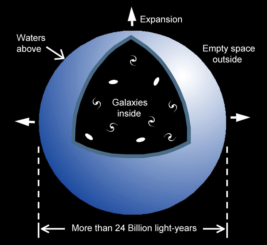
In the fall of 2007 I published a new metric as part of an explanation of the ‘Pioneer anomaly’, a decades-old mystery about the slowing-down of distant spacecraft.⁴ Compared to many modern metrics,⁵ the new one is rather simple. It describes space and time inside an expanding spherical shell of mass. I was interested in that problem because of the ‘waters that are above the heavens’ that Psalm 148:4 mentions as still existing today above the highest stars (see figure 1). The waters would be moving outward along with the expansion of space mentioned in 17 Scripture passages.⁶

According to data in my previous paper, the total mass of the shell of waters is greater than 8.8 × 10⁵² kg, more than 20 times the total mass of all the stars in all the galaxies the Hubble Space Telescope can observe.⁷ However, because the area of the shell is so great, more than 2 × 10⁵³ m², the average areal density of the shell is less than 0.5 kg/m². By now the shell must have thinned out to a tenuous veil of ice particles, or perhaps broken up into planet-sized spheres of water with thick outer shells of ice. It is only the waters’ great total mass that has an effect on us, small but now measurable.

Figure 3. Gravitational potential F inside a spherical shell of mass increases as radius R of the shell increases between two events.

Because of the great mass of the ‘waters above’, I could neglect the smaller mass of all the galaxies in deriving the metric. Although other distributions of mass could also solve the Pioneer mystery, this one seems more applicable to biblical cosmology.

Being relatively simple, the new metric clarifies a new type of time dilation that was implicit in previous metrics but obscured by the effects of motion. This new type, which I call achronicity, or ‘timelessness’, affects not only the narrow volume of space at or just around an ‘event horizon’ (the critical radius around a black hole at which time stops), but all the volume within the horizon. Within an achronous region, we will see, time is completely stopped. I pointed out a related effect, ‘signature change,’ in an earlier paper,⁸ but all I had to go on then was an older metric, the Klein metric, which was quite complicated. The complexity obscured what that metric suggested could happen to time. The cosmology this paper outlines is a new one that does not stem from the Klein metric.

The new metric

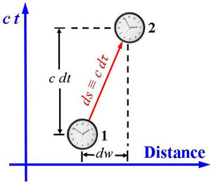
A metric specifies the spacetime interval ds between two events in time and space. When ds is ‘timelike’ (i.e. a real number according to the sign convention I’m using), it is simply c multiplied by the time interval a physical clock would read when moving with the correct speed to cross two events close to each other in space and time:

where dτ is the time interval read out by the clock. The time τ registered by a physical clock (in its rest frame, of course) is called proper time. Figure 2 shows the two events, 1 and 2, a time dt and distance dw apart. As all metrics do, my metric shows how to calculate the spacetime interval ds in a specific situation:⁹

Here dt² and dw² ≡ dx² dy² dz² are the squares of coordinate time and distance intervals, that is, time and length as measured by very distant clocks and rulers where Φ is zero. Notice that dw is not a radial distance interval, but rather a total distance interval with components dx, dy, and dz. So this metric differs from the similar Schwarzschild metric I show later in eq. (16).¹⁰ In this metric, eq. (2), Φ is the gravitational potential¹¹ at any point inside an empty spherical shell of mass M and radius R:

Figure 4. Heavy ring on trampoline illustrates gravitational potential ‘well’.

The radius R can depend on time, making Φ depend on time, and yet metric (2) will still be an exact solution of Einstein’s gravitational field equations. Notice that the potential is a negative number. As applied in this paper, R is the radius (many billions of light-years) of the spherical shell of ‘waters that are above the heavens’ I mentioned in the introduction. As I said in the introduction, R increases with the expansion of space. Eq. (3) shows that as R increases, the potential will get less negative. Figure 3 illustrates that increase.

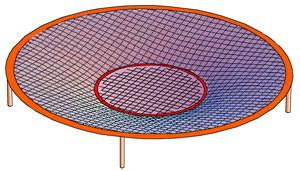
Figure 4 shows an analogy from everyday life, a heavy ring on a backyard trampoline. The two-dimensional ring corresponds to the three-dimensional mass shell of radius R in figures 1 and 3. The dent the ring makes in the fabric of the trampoline has a similar cross-sectional shape as the potential ‘well’ in figure 3. Notice that inside the ring, the trampoline fabric is flat, just as the potential inside R is flat. If we make the ring have a larger diameter, while keeping its weight the same, the dent in the trampoline will get shallower, just as the potential well in figure 3 gets shallower as the radius R gets larger.

Time dilation with the new metric

The metric of eqs. (2) and (3) is exact even for R (hence Φ) changing with time, and for large potentials, even deeper than –c². This exactness allows us to deduce how time dilation depends on gravitational potential and velocity. In terms of coordinate distance and coordinate time, the velocity of the moving clock in figure 2 is:

Insert (1) into (2), divide by c², factor out dt², and use (4) to replace dw/dt:

Take the square root of (5) to get the proper time an object moving with velocity v experiences during an interval of coordinate time dt. That gives us the time dilation:

Notice that for Φ = 0, this equation becomes the velocity time dilation of special relativity:

Eq. (6) is a more general expression, combining the effect of velocity with the effect of gravitational potential.

Time dilation for objects at rest

Consider what happens to a motionless particle. Insert
v = 0 into (6). Then the equation gives a purely gravitational time dilation:

Keep in mind that the potential Φ is a negative number. For shallow potentials, that is, for –c² << Φ ≤ 0, eq. (8) reduces to a simple approximation found in many textbooks:^12,13

Figure 5. Time dilation depends on depth of gravitational potential F.

Notice that the factor 2 disappears along with the square root. Eq. (8) is more useful than eq. (9), because the former is exact even for deep potentials. When the potential is above the critical potential (that is, Φ > F_c, where Φ_c ≡ −½ c²), the expression under the radical (the radicand) in eq. (8) is a positive number. Then proper time τ elapses normally for the particle, but τ becomes slower (with respect to coordinate time t) as Φ approaches the critical potential from above (figure 5). When Φ is exactly at the critical potential, the proper time interval becomes zero. At that point, clocks that are at rest (with respect to the centre) stop.

But what happens as Φ drops below the critical potential, so that Φ < Φ_c? Then the radicand is negative, and we have the proper time interval being the square root of a negative number. That means dτ is a mathematically imaginary number. This suggests that in this region, physical clocks would stop completely. Time would no longer exist. Regions of space below the critical gravitational potential would be achronous.

Achronicity is more extensive than the more familiar kind of time dilation, because the former stops time not in a very narrow region (say just around the event horizon of a black hole) where Φ is close to the critical potential, but throughout possibly vast regions of space, wherever Φ is less than the critical potential. This makes achronicity a much more useful effect for creation cosmology.

The speed of light controls time

This section shows how achronicity is related to the coordinate speed of light, which gives the coordinate distance dw a photon travels during a proper time interval dτ measured by a physical clock at rest in the coordinate frame. (The usual speed of light we measure is different; it gives the physical ruler distance a photon travels during a proper time interval.) In my previous paper,¹⁴ I showed that the coordinate speed of light u_c with my metric is:

The coordinate speed of light is not constant. It can vary from place to place and time to time. That is the underlying cause of the ‘Pioneer anomaly’, according to my previous paper.¹⁵ Most important here: if Φ drops below the critical potential, u_c will become imaginary.

Figure 6. Light-and-mirror clock. Pulsed laser at left makes very short pulse of light. Light enters hole in mirror A and bounces off 99% silvered mirror B, then off mirror A, and so forth many times. Each bounce from mirror B passes 1% of the light pulse through mirror B to photoelectric detector behind it. Output of detector is a series of electrical pulses. Time between output pulses depends on the distance between mirrors and on the speed of light.

Thus in regions of space that are below the critical potential, light cannot propagate. This (as well as many other relativistic effects) suggests a deep connection between the coordinate speed of light and the flow of time. Here are a few reasons for such a connection:

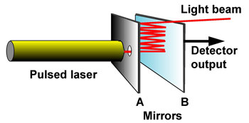
Figure 6 is a diagram of one of the simplest clocks I can imagine, a light pulse bouncing between two mirrors.¹⁶ In a timeless region with no motion of photons, this clock would stop. Simple mechanical clocks depend on c the same way.¹⁷ The speed of light appears to affect all physical processes we understand in the same way. For example, in the relativistic generalization of classical electrodynamics, electric and magnetic forces are proportional to the coordinate speed of light,¹⁸ thus becoming zero or imaginary when the speed becomes zero or imaginary. Or, if you prefer the quantum-mechanical description of electromagnetic forces, particles in an achronous region could not exchange ‘virtual’ photons (the photons being unable to propagate), so they could not interact. No interaction and no forces mean no physical processes and no activity—no time. Thus the coordinate speed of light controls time.

The fabric of space controls the speed of light

Let’s examine what would cause the coordinate speed of light in eq. (10) to become imaginary. Regarding space itself as a real but intangible material,¹⁹ which for biblical reasons²⁰ I call ‘the fabric of space’, Einstein’s famous equation E = mc² suggests a way we can understand. Solve the equation for c and change c to u_c :

where I am regarding E as the energy of a small volume of the fabric of space and m as the inertial mass of the same volume element. Dividing both quantities by the volume gives

where ε is the energy density and ρ is the mass density of the fabric of space at the location. Because Einstein’s equation appears to apply to all forms of energy, I take ε as the total energy density of the volume element. If we are motionless with respect to the fabric of space, the fabric has no kinetic energy in our reference frame. That leaves only the rest mass energy density and the gravitational energy density V of the volume element as the remaining parts of the energy density ε:

Write the gravitational energy density V in terms of the mass density ρ of the volume element and the gravitational potential Φ:

The factor of two is common in relativistic expressions involving potential. For example, it is necessary to get eq. (9) from eq. (8). John A. Wheeler and his colleagues have some interesting comments on this and a relativistic generalization of the concept of gravitational potential.²¹ Use (14) in (13) and insert the result into (12):

This result is the same as eq. (10). The derivation suggests that the coordinate speed of light in a region depends on the total energy per unit mass of the fabric of space in that location. When the gravitational energy of the fabric is negative enough to overcome all other contributions to its energy, light waves can no longer propagate in the fabric, and low-speed physical processes stop. We could regard this effect as a phase change in the fabric of space, analogous to the thermodynamic phase change that occurs when water freezes. The Appendix explains an analogy to this stopping of waves from everyday experience, making a connection between energy density and tension.

Achronicity in previous metrics

The Schwarzschild metric (called his ‘exterior’ metric) I mentioned in the introduction is:

where m is the mass of a non-spinning spherical object at rest, t is the coordinate time, r is a radial coordinate from the centre of the object to a field point in empty space outside the object, and the angles (θ, φ) are colatitude and azimuth. (Outside such an object, the potential and fields are static, and so cannot be applied to the problem of an expanding cosmos with moving masses.) For a clock at rest with respect to the centre of mass, dr, dθ, and dφ are all zero. Using those values and eq. (1) in eq. (16), and then taking the square root gives the time dilation of the motionless clock:

which is the same as eq. (8) with Φ =−Gm/r. For r inside the Schwarzschild radius, r_s ≡ 2Gm/c², i.e. inside the ‘event horizon’ of a black hole but outside the mass, the radicand is negative. So if a particle inside r_s (but outside the mass) could be motionless, it would experience achronicity. However, most relativists think it is impossible for an object to have zero velocity inside the event horizon, partly because they want to avoid the possibility of the spacetime interval ds being imaginary, (i.e. achronicity).²²

Certainly it is quite plausible that the radial velocity of an object would not be zero in the vicinity of the event horizon, because for small and medium-size black holes the acceleration of gravity just outside the Schwarzschild radius would be high (that is, the slope of space is high).²³ In other words, the slope of space in the region is steep. So any object falling into the black hole would have a high speed in the vicinity of r_s.

In that case, v in eq. (6) would be high, allowing dτ to be real even below the critical potential. In other words, the steep slope of space near r_s prevents us from using black holes to detect achronicity, allowing relativists to avoid thinking about that possibility. But the new metric, eq. (2), and its associated time dilation, eq. (6), apply to flat space. That allows objects to be motionless, and thus it confronts us with the question: what happens to motionless objects below the critical potential? The answer I am offering is that time stops.

From 1994 to 2006,²⁴ I was using another metric derived by Oskar Klein in 1961.²⁵ That metric is quite complicated, because in it the fabric of space is usually moving quite rapidly. That means the kinetic energy of the ‘fabric’ is not negligible compared to its rest mass energy and its gravitational potential energy. Even so, under some conditions, all four terms in the metric would turn negative, in which case clocks would be completely stopped regardless of their velocity. The technical term for that phenomenon is signature change. In 1998 I pointed out the possibility of signature change in the Klein metric and the possibility of timelessness.⁸ But this new metric, being simpler, makes the implication of achronicity much clearer. The next few sections outline one scenario showing how timelessness could explain many cosmological observations.

Other forms of the new metric and cosmic redshifts

For cosmology calculations, it is helpful to transform my new metric, eq. (2), into a form similar to the flat or closed-space versions of the Robertson–Walker (RW) metric, the basis of the big bang family of cosmologies.²⁶ First write the distance interval dw in eq. (2) in terms of dimensionless spherical coordinates (χ, θ, φ) that move along with the expansion, as if they were painted onto a rubber sheet that is being stretched out along with the shell of waters of radius R:

These (χ, θ, φ) are co-moving coordinates just like the ones the RW metric uses. Now use eq. (18b) to replace dw² in eq. (2). Then make the transformations

and substitute them into the modified eq. (2). That gives us an RW-like form:

This differs from the RW metric in a very important way: below the critical potential, and S² change sign. However, eq. (20) has the same outward form as the RW metric, so we can, with care, use results derived from the RW metric. For photon trajectories that remain in regions entirely above the critical potential, we can use the textbook derivation²⁷ to get the cosmological redshift implied by eq. (20). That results in a wavelength ratio of:

where l is the wavelength, Φ is the gravitational potential, S is the overall scale factor, R is the radius of the mass shell, and the subscripts 1 and 2 refer to the times of photon emission and reception, respectively. If the potentials at the time and place of emission and reception happen to be the same, eq. (21) reduces to the big bang result. If there is a difference of potential between emission and reception, the redshifts for a constant expansion rate would appear the same as if there had been either an acceleration of deceleration of the expansion. Thus it is easy to have scenarios giving the same redshift-distance relation as the current ‘accelerating’ big bang models. That could do away with not only the need for acceleration of expansion, but also the need for ‘dark matter’ and ‘dark energy’.

Last, insert the following transformation,

into eq. (20), giving the metric in a simple form:

This form implies that if, in regions that are above the critical potential, we plot photon trajectories on a graph with coordinates and, the photon paths will be straight lines inclined at ± 45° angles to the horizontal axis. In the next two sections I will take advantage of that convenient feature to make a spacetime graph explaining how light from distant galaxies could have arrived on Earth quickly, as measured by earth’s clocks.

A fourth-day light transit-time scenario

In this section I outline a speculative light transit-time scenario during Day 4. Other scenarios are possible, so you should take this as only an example of the possibilities that achronicity opens up.

Figure 7. Rising critical potential level makes achronous region expand with velocity vt.

Imagine that events prior to Day 4 have expanded space and moved the shell of ‘waters above the heavens’ out to a radius of, say, one billion light-years.²⁸ Say that this has left the earth and the nearly-flat fabric of space within the waters just above the critical potential.

Now imagine that during the fourth day, God creates star masses in a way that would create a linearly-dented perturbation²⁹ in the otherwise flat potential of the fabric of space, as shown in figure 7. There appear to be several ways to make such a shape.³⁰ But the linear shape is not essential. It only makes illustrating the processes simpler.

As in figure 5, the horizontal dashed line in figure 7 represents the critical potential, Φ_c. As soon as God creates the galaxy masses, the fabric of space begins sinking slowly, and the central part—containing the earth—will drop below the critical potential. An observer in ordinary space a bit farther from the centre would see a black sphere appear around the centre and begin growing in size. According to eq. (8), the entire interior of the sphere is an achronous region. For slow-moving objects in that region, time would be stopped.

The critical potential Φ_c depends on the speed of light, which in turn depends on the tension in the fabric of space (see Appendix). If, as God stretches out the fabric of space (e.g. Isaiah 40:22), He changes the tension simultaneously everywhere, then c will change, and the position of the critical potential with respect to the fabric will also change. (The potential difference ½ c² is anchored to the Φ = 0 axis.) Thus the critical potential line in figure 7 could move up or down quite rapidly.

Let’s suppose the tension in the fabric of space suddenly decreases enough to make the critical potential move upward rapidly. Then sphere of timelessness will expand faster than otherwise. The speed v_t of its expansion (or later, contraction) will depend on three factors: the (inverse of the) radial slope of the potential of the fabric of space (∂Φ/∂r), the rate of the potential’s descent or rise (∂Φ/∂t), and the rate of rise or descent (∂Φ_c/∂t) of the critical potential level:

these factors being evaluated at the location of the surface. For general potential shapes, let’s say that God designs or adjusts these three factors so that the expansion speed v_t of the timeless zone surface is exactly c continuously. (Because the surface of the achronous zone is not a material object, its speed is not limited.) For ∂Φ/∂r constant with radius r, the other two factors can be constant in time to get a constant v_t. For v_t = c, the timeless zone will follow closely behind the wave of galaxy creation, also proceeding outward at the speed of light. As the zone reaches and engulfs each new galaxy, time stops for it.

When the wave of creation stops, say at the location of the waters above, suppose that God now increases the tension, and the critical potential line moves downward. As it does so, the radius of the sphere of timelessness will decrease. Again, let’s imagine that God sets the values of the three factors in eq. (24) to give a contraction speed of –c. As each galaxy emerges from the receding timeless zone, it resumes emitting light. Some of the emitted light will be going inward toward the centre. Because the timeless sphere is moving inward at the speed of light, the inbound light will follow right behind the sphere as it shrinks. When the sphere reaches zero radius and disappears, the Earth emerges, and immediately the light that has been following the sphere will reach earth, even light that started billions of light years away. The stretching of the fabric of space has been occurring continuously all along the light trajectory, thus red-shifting the light wavelengths according to eq. (21).

On Earth, it is still only the fourth day. An observer on the night side of the earth would see a black sky one instant, and a sky filled with stars the next instant. With a telescope he would be able to see distant galaxies having suitably red-shifted spectra.

A second time dilation episode during the Genesis Flood

Figure 8. Timeless zones enable galaxy light to arrive on Earth quickly. Distance and cosmic time are the and of eq. (23). Units of light-years for distance account for the factor c. Scale of the upper, light-coloured timeless zone is exaggerated. Outward-curved trajectories of galaxies are due to expansion of space.

As I have mentioned in several publications,^31,32 two Bible verses lead me to believe that there was a second space-stretching and time dilation episode sometime during the year of the Genesis Flood. One of the verses is Psalm 18:9,

‘He bowed the heavens also and came down with thick darkness under His feet [emphasis added].’

The other verse is 2 Samuel 22:10. It is identical, as the whole chapter is nearly identical to all of Psalm 18. The repetition suggests that the psalm is quite important. In it David reminisces about how the Lord has rescued him from dangers. In this section of the psalm, he speaks in terms of a cataclysmic event that appears to be the Genesis Flood. Everywhere else in Scripture, the phrase here translated ‘bowed the heavens’ is translated as ‘stretched out the heavens.’ The primary meaning of the Hebrew verb, natah, is ‘stretched.’ The translation ‘bowed’ is far down the list of possible secondary meanings.³³ So I prefer the primary meaning, which suggests that God stretched out space out at a higher-than-usual speed (as measured on Earth) during the Genesis Flood.

Scientific considerations applying to the Flood suggest to me that time dilation occurred during this event of space stretching, and it helps explain why the stretching would appear to be very rapid as seen from Earth.³⁴

Figure 8 is a spacetime diagram showing both time dilation events, one of large spatial extent (gray region) occurring during Day 4, and the other of lesser extent (upper, lighter-coloured triangular region) occurring 1656 years later during the year of the Genesis Flood. The expansion and contraction of the lighter-coloured region is slower than the speed of light, and it only extends out to, say, a few hundred thousand light-years. At one instant during the flood year, if Noah could have seen the night sky, its appearance would have changed suddenly. With a suitable telescope, he would have seen the galaxies suddenly look roughly 500 Ma older (i.e. spiral galaxies would be more wound up, etc.). The second dilation event, combined with the speed-of-light recession speed of the achronous zone, explains why distant galaxies, especially spiral galaxies, look no younger than nearby ones. This scenario illustrates the usefulness of achronicity.

Conclusion

The new metric I derived in 2007 has yielded several interesting results. One is a straightforward explanation of the Pioneer anomaly. In this paper, it has revealed a new type of time dilation, achronicity. The fundamental cause of achronicity appears to be that gravitational potential becomes so negative that the total energy density of the fabric of space becomes negative. That stops the propagation of light, all physical processes, and all physical clocks, thus stopping time itself.

I have examined the effect only for essentially motionless bodies (having velocities very much less than that of light). In a later paper, I hope to explore some of the interesting and possibly useful effects of achronicity for non-negligible particle velocities. The speculative scenario in the previous two sections shows how useful achronicity could be in creation cosmology. Other scenarios are easily possible, and I hope that other creationists making alternative cosmologies will find timelessness a good tool.

APPENDIX: An analogy from everyday experience

A stretched string³⁵ (or an elastic sheet³⁶) propagates transverse waves with a speed

where ρ is the mass per unit length (or area), and T is the tension, the force (or the force per unit length) tending to pull the string (or sheet) apart. I like to demonstrate this with a heavy cable (which has a high mass per unit length) tied to a tree. Stand many metres away from the tree with the cable lined up horizontally with your line of sight and pull the cable horizontally toward you to give it some tension. Now give it a sharp jerk up and down, just once. You will see a vertical pulse travel along the cable to the tree, bounce off it, and return toward you.

The harder you pull the cable toward you, increasing the tension, the faster the pulse will travel. If you decrease the tension, the wave travels slower. If you did the experiment in space, in zero gravity, you could decrease the tension to zero and the cable would not droop. But with zero tension, the wave speed would be zero.

If, still in space with no gravity, you then pushed on the end of the cable a little, you would be applying negative tension, i.e. pressure, upon it. The cable might bend a little, but there would be no force trying to restore it to straightness. That means transverse motions would not move along the cable, resulting in no wave propagation. The transverse wave velocity u_s in eq. (A1) would be mathematically imaginary. Just as negative tension in the cable (or sheet) stops waves from propagating along it, so also negative total energy in the fabric of space stops light from propagating through it.

Table 1. Analogy between transverse mechanical waves and electromagnetic waves.

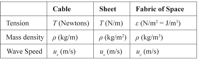
Thus there is a close correspondence between eqs. (12) and (A1), and the meaning of a negative radicand in the two equations is the same—no wave motion. Table A1 summarizes the analogy between the two equations.

Notice that the energy density ε at the top of the right-hand column is analogous to the tension T in the previous two columns. For the 3D fabric of space, dimensional analysis shows that the units of tension (Newtons per square metre) are the same as the units of energy density (Joules per cubic metre). So this analogy makes a connection between the tension in a fabric and the total energy density of space.

The analogy extends even further. As figures 3 and 4 showed, there is a close correlation between the depression caused by a weight on a two-dimensional stretched membrane and the potential in Newtonian (three-dimensional) or Einsteinian (four-dimensional) gravity. I have found this analogy to be very fruitful in understanding the physical meaning behind the mathematics of general relativity.

Related articles

• Creationist cosmologies explain the anomalous acceleration of Pioneer spacecraft
• Dark matter and a cosmological constant in a creationist cosmology?

Further reading

• Astronomy and Astrophysics Questions and Answers

Related resources

Starlight and Time DVD

by Dr. Russell Humphreys

Learn how practical physics using Einstein’s relativity explains how light could be seen on Earth during Creation week. Dr Russell Humphries presents over 2 hours of footage, including stunning 3-D graphics in support of the Bible’s account of creation. (High School-Adult) 140 mins. While the content of this popular, illustrated presentation DVD is the same as one you may have with the same title, it now includes extra features. Not only does it have a new cover design, it has also been ‘re-badged’ to feature the CMI logo and contact details and includes a 3-minute promotional segment.

Starlight, Time and the New Physics

by Dr. John Hartnett

Written by Dr John Hartnett, this is a bold new answer to the distant starlight issue. Many still doubt the Bible’s clear timescale because, they think, it is impossible for light to have reached the Earth in only a few thousand years from stars that are millions of light-years away. This misconception is often the ultimate stumbling block to a straightforward acceptance of the Bible—even the gospel itself. Understandable by intelligent laypersons, with technical equations and papers put into 111 pages of appendices for the specialist. (High School–Adult) 231 pages.

References

1. Humphreys, D.R., Creationist cosmologies explain the anomalous acceleration of Pioneer spacecraft, Journal of Creation 21(2):61–70, August 2007, eqs. (9) and (A59). Archived at <creationon.com/images/journal_of_creation/vol21/5181creationist.pdf>. Return to text.
2. Einstein, A., Zur allgemeinen Relativitätstheorie, Sitzungsberichte der Preussischen Akademie der Wissenschaften Berlin (About the General Theory of Relativity, Proceedings of the Prussian Academy of Science Berlin), pp. 778–786, 1915. English translation of similar 1916 Einstein paper in: Lorentz, H.A., Einstein, A., Minkowski, and Weyl, H. The Principle of Relativity, Dover Press, pp. 111–164, 1952. Return to text.
3. Schwarzschild, K., Über das Gravitationsfeld eines Massenpunktes nach der Einsteinschen Theorie, Sitzungsberichte der Preussischen Akademie der Wissenschaften Berlin (On the gravitational field of a point mass according to the Einstein theory), pp. 189–196, 1916. Schwarzschild derived his metric while serving as a soldier on the German east front during World War I, where he died later the same year. Return to text.
4. Humphreys, ref. 1. See appendix of the paper for derivation of the new metric. Return to text.
5. Hawking, S.W. and Ellis, G.F.R., The Large Scale Structure of Space-Time, Cambridge University Press, Cambridge, pp. 156–179, 1973, describing the Reissner-Nordström, Kerr, Gödel, Taub-NUT, and other metrics. Return to text.
6. Humphreys, D. R., Starlight and Time, Master Books, Green Forest, AR, p. 66, 1994. See 2 Sam. 22:10; Job 9:8, 26:7, 37:18; Psalm 18:9, 104:2, 144:5; Isaiah 40:22, 42:5, 44:24, 45:12, 48:13, 51:13; Jer. 10:12, 51:5; Ezek. 1:22; Zech. 12:1. Return to text.
7. Humphreys, ref. 1, p. 64. Return to text.
8. Humphreys, D.R., New vistas of space-time rebut the critics, Journal of Creation 12(2):195–212, August 1998. Archived at <www.trueorigin.org/rh_connpage2.pdf>. Return to text.
9. Humphreys, ref. 1, eqs. (9) and (A59). Return to text.
10. Humphreys, ref. 1, p. 68, eqs. (A58) and (A59). That is, even if we were to put Φ = –GM/r into eq. (2) and change to spherical coordinates as in eq. (A58) of this reference, we still would not get eq. (16), which has the factor (1 + 2GM/c² r)^–1 in only one of its three spatial terms. Return to text.
11. Gravitational potential Φ at a point is the energy needed to lift a unit test mass from the point up to a reference location where Φ is defined as zero. In this paper the reference location is far outside the shell of waters (the potential approaches zero inversely with distance in that region) and thus far above all other mass in the cosmos. Return to text.
12. Landau L.D., and Lifshitz, E.M., The Classical Theory of Fields, 4th revised English edition, Pergamon Press, Oxford, p. 248, eq. (88.2), 1983. Return to text.
13. Humphreys, ref. 6, p. 102, eq. (10). Return to text.
14. Humphreys, ref. 1, p. 63, eq. (14) with r → w. Return to text.
15. Humphreys, ref. 1, p. 70, end note 35. Return to text.
16. Humphreys, D.R., C decay and galactic red-shifts, Journal of Creation 6(1):74–79, April 1992. Return to text.
17. Humphreys, D.R., Has the speed of light decayed recently? Creation Research Society Quarterly 25:40–45, June, 1988. See esp. the rotating-mass clock of figure 3, p. 44, which would slow in exact proportion to a slowing of c. Return to text.
18. Landau and Lifshitz, ref. 12, pp 257–258. Note that h ≡ g₀₀ = coordinate speed of light squared, and note the last sentence on p. 258, saying that in this case both the electric permittivity ε₀ and magnetic permeability µ₀ of space are both equal to 1/√ h. That means, for example, that the factor 1/4p ε₀ in the SI form of the Coulomb force equation is proportional to the coordinate speed of light. Return to text.
19. Humphreys, ref. 6, pp. 66–68, 84, 89–90. Return to text.
20. Humphreys, ref. 6, pp. 66–67, noting the Scriptural comparisons of space (the heavens) to a curtain, a tent curtain, a tent, a mantle, a garment, etc. Return to text.
21. Harrison, B.K., Thorne, K.S., Wakano M. and Wheeler, J.A., Gravitation Theory and Gravitational Collapse, University of Chicago Press, Chicago, IL, pp. 19–23, 1965. Return to text.
22. Rindler, W., Essential Relativity: Special, General, and Cosmological, Revised 2^nd edition, Springer-Verlag, New York, Section 8.5, p. 149, 1977. Return to text.
23. Ibid, pp. 148–149, eq. (8.71). Return to text.
24. Humphreys, ref. 6, pp. 115–116, eqs. (16) through (18). Return to text.
25. Klein, O., Einige probleme der allgemeinen Relativitätstheorie (some problems of the General Theory of Relativity); in: Bopp, F. (Ed.), Werner Heisenberg und die Physik unserer Zeit (Werner Heisenberg and the physics of our time). Vieweg & Sohn, Braunschweig, pp. 58–72, 1961. In German. Return to text.
26. Landau and Lifshitz, ref. 12, pp. 358–362, eq. (112.2). Return to text.
27. Narlikar, J. V., Introduction to Cosmology, 2^nd edition, Cambridge University Press, Cambridge, England, pp. 92–94, 1993. Return to text.
28. Humphreys, ref. 6, pp. 76–77. Also see Genesis 1:6. Return to text.
29. It is not hard to show that a small perturbation added to the flat potential of eq. (3) and then used in metric (2) is at least an approximate solution of the Einstein field equations, as it would be for the Newtonian equations. Thus the perturbed-potential metric would have the same general features as the flat metric, particularly having the possibility of achronous regions. Return to text.
30. Humphreys, ref. 1, p. 69, end note 25. One way to make a linear dent in the potential, according to rough calculations of mine, is to create the galaxies in a wave proceeding outward from the centre at the speed of light. Another way is to create all the galaxies simultaneously with a number density decreasing inversely with distance away from the centre. As I mentioned in the text, the linearity of the dent is not necessary; it only makes the illustration simpler. Return to text.
31. Humphreys, ref. 6, p. 68. Return to text.
32. Humphreys, D. R., Accelerated nuclear decay: a viable hypothesis? in Radioisotopes and the Age of the Earth, Vol. I, Vardiman, L., Snelling A.A. and Chaffin, E.F., editors, Institute for Creation Research, El Cajon, CA and Creation Research Society, St. Joseph, MO, pp. 333–379, 2000. See esp. pp. 367–368. Book downloadable at no cost as a 2.5 MB PDF from <www.icr.org/i/pdf/research/rate-all.pdf>. Return to text.
33. Brown, F., The New Brown-Driver-Briggs-Genesius Hebrew and English Lexicon, Hendrickson Publishers, Peabody, MA, pp. 639–640, entry 5186, natah, 1979. Return to text.
34. Humphreys, D.R., Young helium diffusion age of zircons supports accelerated nuclear decay, in Radioisotopes and the Age of the Earth, Vol. II, Vardiman, L., Snelling A.A. and Chaffin, E.F., (Eds.) Institute for Creation Research, El Cajon, CA and Creation Research Society, Chino Valley, AZ, pp. 25–100, 2005. See esp. pp. 70–74. Return to text.
35. Morse, P.M., and Feshbach, H., Methods of Theoretical Physics, Vol. I, McGraw-Hill Book Company, New York, pp. 120–124, eq. (2.1.9), 1953. Return to text.
36. Elmore, W. C., and Heald, M. A., Physics of Waves, Dover Publications, New York, pp. 50–52, eqs. (2.1.1) and (2.1.2), 1985. Return to text.