

Journal of Creation 31(1):88–98, April 2017
Browse our latest digital issue Subscribe
A broken climate pacemaker?—part 1
The results from the well-known “Pacemaker of the ice ages” paper, which convinced uniformitarian scientists of the validity of Milankovitch climate forcing, are now largely invalid, due to a significant revision in the age of the Brunhes–Matuyama magnetic reversal boundary. Unfortunately, the Blackman–Tukey method used to obtain both the original and new results is somewhat obscure. Because of the important role that Milankovitch theory plays in both geochronology and ‘climate change’ speculation, it would be helpful if there were a simple way that other scientists, and even nonspecialists, could confirm these new results without the need for extensive computation. Here I summarize the results of these new calculations and present a simple conceptual argument that allows others to partially verify these results, using only a pocket calculator or an Excel spreadsheet. This would make an excellent critical thinking exercise for high school or middle school science or mathematics students.

Milankovitch climate forcing is now the dominant secular explanation for the fifty or so Pleistocene glacial intervals (‘ice ages’) said to have occurred within the last 2.6 Ma.1 This theory posits that changes in the seasonal and latitudinal distribution of sunlight, resulting from variations in Earth’s orbital motions, pace the Pleistocene ice ages. In particular, these climate changes are thought to result from variations in the elongation of the earth’s orbit (eccentricity), the tilt of the earth’s axis (obliquity), and the longitude of the earth’s perihelion (point of closest approach to the sun), measured with respect to the vernal equinox. The concept of Milankovitch climate forcing has numerous problems2–5 but is today largely accepted because of a well-known 1976 paper titled, “Variations in the earth’s orbit: the pacemaker of the ice ages”.6 The paper’s authors, James Hays, John Imbrie, and Nicholas Shackleton, performed spectral analyses on three quantities (of assumed climatic significance), sampled at 10 cm intervals, within two deep-sea sediment cores from the southern Indian Ocean. The cores were designated as RC11-120 (length of 9.5 m) and E49-18 (length of 15.5 m). A third core, designated as V28-238, in the western Pacific Ocean, played an important, but indirect, role in the analysis (figure 1). Analyses of the oxygen isotope data (discussed below) and other variables showed climate cycles having periods of approximately 100, 42, and 23 thousand years (ka). Because the lengths of these cycles corresponded well to those of inferred cycles in Earth’s orbital and rotational motions, the Pacemaker paper was seen as providing strong support for the Milankovitch theory.

Experts acknowledge that evidence for the Milankovitch (or astronomical) theory comes almost exclusively—if not exclusively—from spectral and/or time series analyses performed on paleoclimate data, like those performed in the Pacemaker paper. Physicist Richard Muller and geophysicist Gordon MacDonald noted:
“In fact, the evidence for the role of astronomy [in climate variation] comes almost exclusively from spectral analysis. The seminal paper was published in 1976, titled, ‘Variations of [sic] the earth’s orbit: pacemaker of the ice ages.’”7
Likewise, noted physicist Walter Alvarez stated:
“The widely accepted Croll-Milankovitch theory that fluctuating climate conditions during the Quaternary glaciation have been driven by astronomical cycles is based entirely on time-series analysis of paleoclimatic and orbital data [emphasis added].”7
Implications for geochronology and the ‘climate change’ debate
This paper argues that the original results presented in the Pacemaker paper are invalid, even by uniformitarian reckoning. Before discussing why this is the case, it is good to explain why this is significant.
The Milankovitch theory has become an extremely important aspect of secular geochronology. Uniformitarian scientists now generally assume the theory to be valid and use that assumption to assign relatively ‘young’ ages (thousands of years to a few million years) to deep-sea sediment cores via a technique called ‘orbital tuning’.8 These ages are then used to assign ages to other deep-sea cores, as well as the deep ice cores of Greenland and Antarctica.9 Likewise, uniformitarian scientists are now using the Milankovitch theory in an attempt to assign ages even to Triassic sediments.10 Incredibly, the Milankovitch theory is even used to assign ages to the dating standards used in argon-argon dating.11,12 If the evidence for the Milankovitch theory is weak, then all of these age assignments are called into question—even by uniformitarian reckoning. The consequences to uniformitarian geochronology would obviously be devastating.
Likewise, the Milankovitch theory is making a subtle contribution to ‘climate change’ alarmism, a subject which is discussed in more detail in part 2 of this series.13
Pacemaker problems


However, there are serious problems with the Pacemaker paper.14-16 First, multiple versions of the data from these two cores exist, raising the question, which versions are the ‘real’ ones? Most of the differences between data sets are trivial, but in some cases, data points (and even small blocks of data) used in the original Pacemaker analysis have been removed from the newer versions of the data.17 Furthermore, the original 10-cm resolution data actually used by the Pacemaker authors do not seem to be publicly available. I requested these data from the two surviving Pacemaker authors, but they did not respond to those requests. Hence, in order to replicate their results, I had to carefully reconstruct the data from figures 2 and 3 in the original Pacemaker paper. I have compiled these different data versions into tables in order to facilitate side-by-side comparisons of the older and newer data sets.18
Second, the Pacemaker authors excluded from their analysis all data from depths above 4.9 m within the E49-18 core, probably needlessly. In fact, they did not even bother to plot the oxygen isotope data for depths above 3.5 m (figure 3 in the original Pacemaker paper) in the E49-18 core! The purported justification for this exclusion of data was that the age at the top of the E49-18 core was uncertain (and possibly as old as 60,000 years), making the upper third of the E49-18 core unusable for analysis.19 However, other secular scientists disagreed, arguing that the top of the core was quite young.20 That would imply that the upper section of the E49-18 core was potentially datable by the radiocarbon method (even within a uniformitarian framework), which would mean that the uppermost E49-18 data were indeed usable for their analysis.
Third, before performing their analyses, the Pacemaker authors had to assign tentative timescales to the two cores. Critical to these timescales, especially for the longer E49-18 core, was an assumed age of 700 ka for the most recent magnetic reversal boundary, the Brunhes–Matuyama (B–M) magnetic reversal boundary. This age was based on K-Ar dating of volcanic rocks which recorded this reversal.21 However, uniformitarian scientists have since revised the age of the B–M reversal boundary upward to 780 ka.22–24 Incredibly, it seems that uniformitarian scientists never bothered to see what effect this age revision would have on the original Pacemaker results!
I have recently reperformed the Pacemaker frequency domain calculations, using the same method as the paper’s authors, but taking into account this revision to the age of the B–M reversal boundary, as well as the inclusion of the previously excluded data from the second core. These changes dramatically weaken, if not completely invalidate, the original argument for Milankovitch climate forcing presented in that paper.16
In order to understand the original and new Pacemaker results, it is necessary to consider some background material.
Foraminifera, oxygen isotope ratios, and marine isotope stages
Microscopic marine organisms called foraminifera construct shells composed of calcium carbonate, CaCO3. When these organisms die, their remains become part of the debris accumulating on the seafloor. Scientists often measure the amount of 18O in a foraminiferal shell compared to the amount of 16O and calculate a quantity called the oxygen isotope ratio, denoted by the symbol δ18O.
If one plots δ18O values from a sediment core as a function of depth, many ‘wiggles’ are readily apparent (figures 2 and 3). These oxygen isotope values are thought to be global climate indicators: maximum values of δ18O within seafloor sediments are thought to indicate times at which global ice volumes were largest, and minimum δ18O values are thought to indicate times when global ice volumes were smallest.25
Because uniformitarian paleoclimatologists think that the δ18O signal is a global climate indicator, they believe that the same basic pattern of δ18O wiggles present in one core should be present in other cores. Of course, they recognize that changes in sedimentation rate, local weather effects, etc., can alter or distort this signal. Nevertheless, they believe that it is possible to ‘match’ δ18O features within one core to corresponding δ18O features in another core, even if the two cores are separated by great distances. Hence, they believe it is possible to transfer ages assigned to prominent δ18O features within one core to (presumed) corresponding δ18O features in another core.
To facilitate this wiggle-matching process, uniformitarian scientists have invented a numbering system involving marine isotope stages (MIS). Our present-day climate is part of MIS 1, which includes the so-called Holocene epoch. The most recent ice age corresponds to MIS 2-4, and most of MIS 5. MIS 5 was originally classified entirely as an interglacial, but secular paleoclimateologists now restrict the interglacial classification to the earliest δ18O ‘trough’ within MIS 5, substage MIS 5e.26 Likewise, MIS 6 corresponds to the penultimate (second-to-last) ice age. Generally, the boundaries between marine isotope stages occur at the depths at which the δ18O values have transitioned halfway from a very low to a very high δ18O, or vice versa. The oxygen isotope values from the RC11-120 and E49-18 sediment cores are shown in figures 2 and 3, along with the approximate MIS boundary locations.
Age assignments for marine isotope stage boundaries
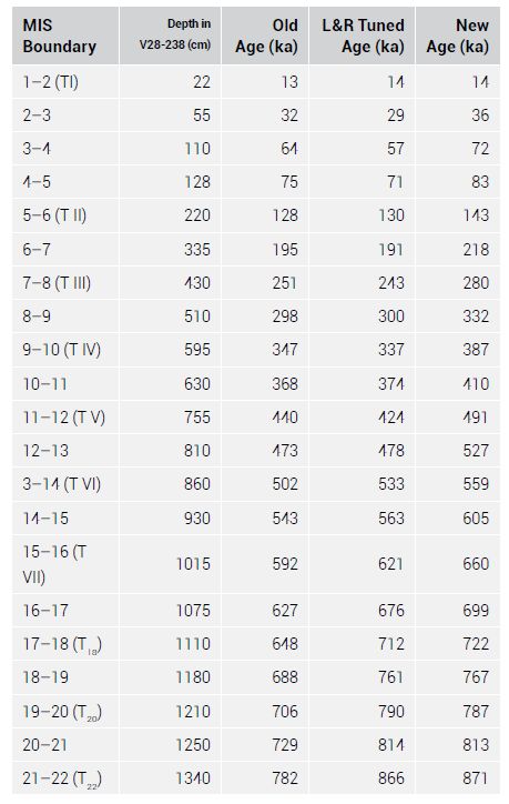
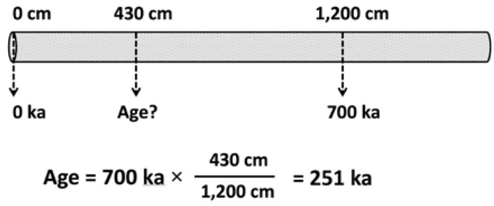
Before the Pacemaker authors could analyze the RC11-120 and E49-18 data, they had to assign timescales to these two cores. Radioisotope dating methods cannot generally be used to date the deeper sediments (although protactinium-thorium dating is theoretically capable of dating sediments thought to be less than 175,000 ka old27), and uniformitarian scientists believe that radiocarbon dating methods can only be used on the uppermost sediments. Hence, uniformitarian scientists used the long western Pacific V28-238 core to indirectly assign ages to the sediments. They chose this particular core because it was believed to have the most nearly constant sedimentation rate of all the cores that had been examined.28 Magnetic minerals within the sediments showed a reversal of the earth’s magnetic field at a depth of 1200 cm within the V28-238 core. Uniformitarian scientists had already used K-Ar dating to assign an age of 700 ka to volcanic rocks showing this same reversal. Hence, they concluded that the sediments at a depth of 1200 cm within the V28-238 core were 700 ka old. By assuming that the top of the V28-238 core had an age of 0 ka and that the seafloor sediments at that location had accumulated at a nearly constant rate, they were able to assign tentative ages to the first 21 MIS boundaries within the core (figure 4).29 The results of these calculations are shown in table 1 (third column from left), as are the results if one changes the assumed age of the B–M reversal from 700 ka to 780 ka (far right column).
The Pacemaker authors transferred the age assignment of 440 ka for the MIS 12-11 boundary, the age assignment of 251 ka for the MIS 8-7 boundary, and the age assignment of 128 ka for the MIS 6-5 boundary to the presumed corresponding MIS boundaries in the RC11-120 and E49-18 cores. Technically, however, the Pacemaker authors did not actually use this last age estimate of 128 ka in their analysis. Protactinium-thorium dating applied to the V12-122 Caribbean core had already yielded an age estimate of 127 ka for the MIS 6-5 boundary, and the Pacemaker authors felt that this slightly lower age estimate was a little more accurate.30 They no doubt, however, considered the close agreement between these two age estimates of 127 ka and 128 ka to be a confirmation of the validity of their assumption of a (nearly) constant sedimentation rate within the V28-238 core.
They then used these three-age control (or anchor) points to construct timescales for the two sediment cores. For their initial analysis, they employed simple timescales (which they dubbed as ‘SIMPLEX’), utilizing only two age control points within each core and the assumption of a constant sedimentation rate. Within the RC11-120 core, the MIS 6-5 boundary was identified at a depth of 4.40 m. Hence, an age of 127 ka was assigned to this depth in the RC11-120 core. An age of 0 ka was assumed for the top of the RC11-120 core, and ages were assumed to increase at a constant rate with depth within the core.
As noted earlier, they completely excluded the upper third of the E49-18 core from their analysis. The MIS 6-5 boundary was identified at a depth of 4.90 m within this second core; hence the age of 127 ka was assigned to this depth. The MIS 12-11 boundary was identified at a depth of 14.05 m; hence, this depth within the E49-18 core was assigned an age of 440 ka. Again, age was assumed to increase linearly with depth down the core.
Spectral analysis


Figure 5 shows the manner in which three waves of different frequencies, amplitudes, and phase constants may be added (superposed) together to yield a composite waveform. Although the number of waves needed to construct the δ18O waveforms shown in figures 2 and 3 is much larger, the principle is the same: these complicated waveforms may also be constructed by adding together waves of different frequencies, amplitudes, and phase constants. It is also possible to ‘reverse-engineer’ the waves that have been superposed in order to obtain the final resulting waveform. This is the rationale behind spectral analysis, in which composite waveforms are decomposed into their constituent waves. A Discrete Fourier Transform (DFT) may be used for this purpose. However, the DFT is subject to some weaknesses, discussed briefly below, which makes it less than ideal for such an analysis.31 After assigning their SIMPLEX timescales to the two Indian Ocean sediment cores, the Pacemaker authors used the Blackman–Tukey method32 to analyze the three variables that had been measured in the cores: the δ18O values of the planktonic foraminiferal species Globigerina bulloides, the percent abundance of one particular radiolarian species (Cycladophora davisiana) relative to the other radiolarian species, and (southern hemisphere) summer sea surface temperatures (also inferred from radiolarian data). Their analysis resulted in graphs called power spectra. A power spectrum is a graph consisting of peaks of varying height, plotted against frequency. Prominent peaks occur at the frequencies corresponding to large-amplitude waves making a large contribution to the overall signal.33 One of the difficulties with a DFT is that spurious peaks often appear in the resulting power spectra. The Blackman- Tukey method, on the other hand, alleviates this difficulty. Likewise, the Blackman-Tukey method is a good choice when the timescale is uncertain, as in the Pacemaker analysis. The results from their original spectral analyses are shown in figure 5 of the original Pacemaker paper, as well as in figures 9–17 in my second paper.34,35 Comparison of these graphs show generally good agreement between my results and theirs, despite the fact that I obtained my results using a reconstructed data set.36
Figure 6 depicts the original δ18O power spectrum results for a composite ‘core’ called PATCH which the Pacemaker authors constructed using the uppermost RC11-120 data and the lowermost E49-18 data. This power spectrum was calculated for the time interval 0 to 486 ka. In the original Pacemaker paper, the authors used a relatively small number (51) of discrete frequencies when calculating their power spectra. However, experts cited by the Pacemaker authors claim that one can legitimately use 2–3 times as many discrete frequencies as did the Pacemaker authors.37 I have taken the liberty of doing so, as well as ‘zooming in’ on the pertinent part of the spectrum. The vertical lines in figure 6 indicate the eccentricity, obliquity, and precessional frequencies calculated by the Pacemaker authors. The peaks align well with the vertical lines, indicating good agreement between the results and Milankovitch expectations (even though the last vertical line does not pass directly through the centre of the C peak, this can still be reasonably counted as a ‘hit’ for the theory).
Figure 7 shows the same δ18O power spectrum, but after taking into account the revised age of 780 ka for the B–M magnetic reversal boundary. The new time interval corresponding to the PATCH ‘core’ extended from 0 to 544 ka. The vertical lines in figure 7 indicate the eccentricity, obliquity, and precessional frequencies I calculated using the B-T method and the astronomical data for the interval 0 to 544 ka.38,39
Note that the age revision has noticeably shifted the locations of the smaller B and C peaks in figure 7 (corresponding to the obliquity and precession frequencies, respectively) so that those peak frequencies no longer agree with frequencies expected by the Milankovitch theory.
This age revision also shifts the results for the RC11-120 core and the bottom section of the E49-18 core.
Spectral analysis performed using all the data from the E49-18 core (including the originally excluded section) also yielded results that were generally in poor agreement with Milankovitch expectations.16
Verifying the results
Because these calculations require integral calculus and a computer, laypeople may not have the technical expertise to use the Blackman–Tukey method to verify these results. Furthermore, those who do have the necessary expertise may simply not have the time to check the results. Given the potential importance of these results for geochronology and the ‘climate change’ debate (discussed in a second paper), is there a way that others can at least partially test them (which we are enjoined to do in 1 Thessalonians 5:21)?
Yes. First, one can easily verify both the old and new estimated ages for the MIS boundaries (table 1) using the method shown in figure 4. Also, these new age estimates introduce an apparent cause-and-effect problem. The original MIS boundary age estimates (at least those for the twelve most recent boundaries identified in the two Indian Ocean cores) were reasonably close to tuned ages (second column from right in table 1) that were based on a simple ice model tied to summer insolation at 65°N:40 nearly all the discrepancies between the two methods were less than 10 ka. However, after the age revision for the B–M reversal boundary, six of these twelve age estimates are now at least 32 ka greater than expected, based on Milankovitch expectations, and one (the MIS 12-11 boundary) is 67 ka greater than expected! This raises a question: how can the climate be changing multiple tens of thousands of years before the changes in summer insolation that supposedly caused the changes?
Likewise, one may use simple algebra and the two SIMPLEX age control points within the RC11-120 core to show that the original RC11-120 SIMPLEX ages (in ka), as a function of depth (in metres), are given by
ageRC11-120 (original) = (28.864 ka/m) × depth (1)
Likewise, the original SIMPLEX ages (in ka) for the bottom two-thirds of the E49-18 core are given by
agebottom of E49-18 (original)= (34.208 ka/m) × depth – 40.619 ka (2)
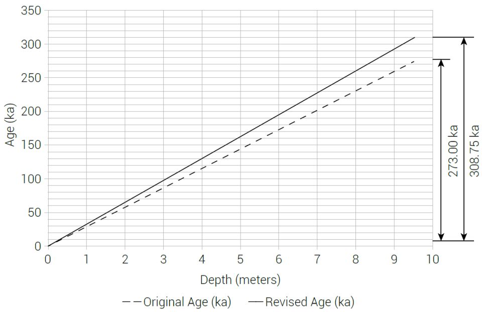
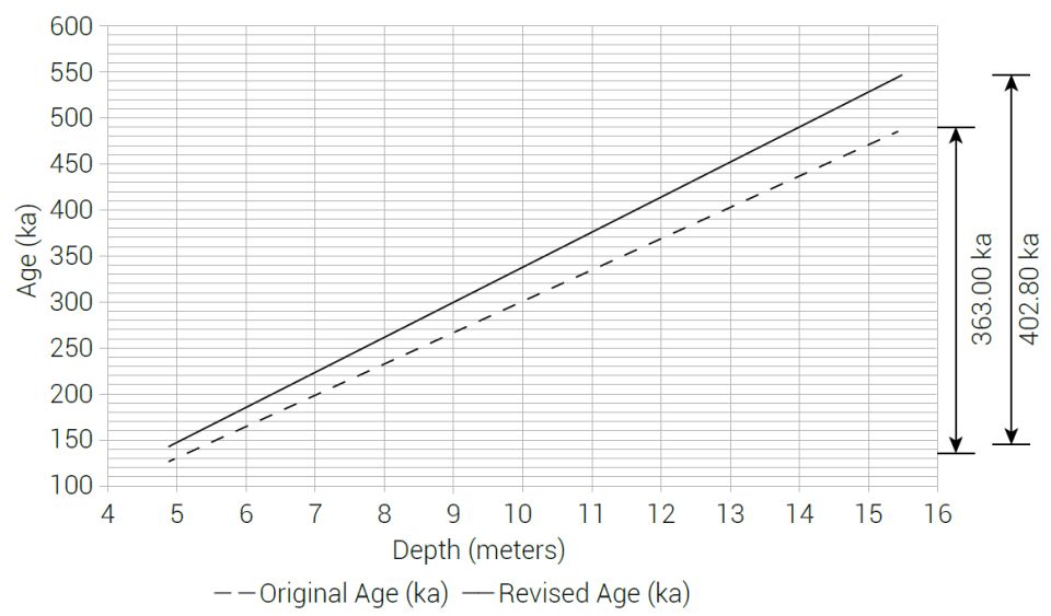
Inserting depths of first 0.0 m and then 9.50 m into Eq. (1) enables one to show that the ages corresponding to the top and bottom of the RC11-120 core are, respectively, 0.0 ka and 274.2 ka. Hence the total time assigned to the length of the RC11-120 core is 274.2 ka – 0.0 ka = 274.2 ka. Likewise, inserting depths of 4.9 m and 15.5 m into Eq. (2) allows one to verify that the length of time assigned to the bottom section of the E49-18 core is 489.6 ka – 127.0 ka = 362.6 ka. Even though the preliminary timescales used in the Pacemaker analysis assume a constant sedimentation rate, round-off error may cause the time increments between data points to vary slightly. Because the Blackman–Tukey method requires evenly spaced data points, the Pacemaker authors had to specify a time increment Δt and then interpolate the data so that the total time intervals were integer multiples of Δt. They chose their time increment Δt to be 3 ka for both cores. Hence, the time intervals for the core sections, after interpolation, were 273 and 363 ka (figures 8 and 9, respectively). This corresponded to 92 interpolated data points for the RC11-120 core and 122 interpolated data points for the bottom section of the E49-18 core.
New timescales
Of course, the revised age of 780 ka for the B–M reversal boundary alters the ages for the MIS boundaries, which, in turn, alters Eqs. (1) and (2). The original age estimates of 127 and 128 ka for the MIS 6-5 boundary were in good agreement with one another, but the revised age of 780 ka for the B–M reversal boundary yields an age estimate of 143 ka for this boundary, resulting in an apparent discordance between the two age estimates. Someone hoping to salvage at least some of the original Pacemaker results might think that the age of 127 ka would be the better choice, as this would leave the original RC11-120 results unaffected by the age revision. However, the RC11-120 results are apparently not statistically distinguishable from the background noise.41 Hence, they are not, in and of themselves, a convincing argument for Milankovitch climate forcing.
What about the E49-18 core? The new age of 780 ka for the B–M reversal boundary and the method of Shackleton and Opydke (table 1) implies an age estimate of 279.5 ka for the MIS 8-7, as well as an age estimate of 490.75 ka for the MIS 12-11 boundary. But the B–M reversal boundary in the V28-238 core was apparently the only means available to the Pacemaker authors to assign ages to the MIS 8-7 and 12-11 boundaries. For this reason, the oxygen isotope signal in the V28-238 core was extremely important to secular paleoclimatologists and has been called an ice age ‘Rosetta Stone’.42 Hence, if one wants to redo the calculations for the E49-18 core using the method of the Pacemaker authors (but after taking into account the age revision to the B–M reversal boundary), he has no choice but to use these new age estimates for the MIS 8-7 and 12-11 boundaries. But if one is willing to trust this method to obtain age estimates for the MIS 8-7 and 12-11 boundaries, then logically one should also be willing to use that method to obtain an age estimate for the MIS 6-5 boundary. Hence, the pragmatic (but not necessarily scientifically objective!) choice would be to go ahead and use the age estimate of 143 ka for the MIS 6-5 boundary, despite the resulting apparent cause-and-effect problem.
The new age estimates (as a function of depth) within the two cores are given by
ageRC11-120 (new) = (32.5 ka/m) × depth (3)
agebottom of E49-18 (new) = (38.005 ka/m) × depth – 43.227 ka. (4)
One can verify that Eq. (3) yields an age of 0 ka at the top of the RC11-120 core and an age of 143 ka at a depth of 4.40 m in the RC11-120 core, as should be the case. Likewise, Eq. (4) yields an age estimate of 143 ka at a depth of 4.90 m within the E49-18 core, and an age of 490.75 ka at a depth of 14.05 m, also as expected. The age for the MIS 8-7 boundary was not used in these calculations, as it was only used later to construct the ‘ELBOW’ chronology for the ‘PATCH’ core (table 2 in the Pacemaker paper).
One can also use Eqs. (3) and (4) and to verify that the new total time (prior to interpolation) assigned to the RC11-120 core is 308.75 ka and that the new time assigned to the bottom section of the E49-18 core is 402.85 ka.
When redoing the Pacemaker calculations, I attempted to minimize interpolation as much as possible, as it is always preferable, if possible, to perform the analysis on the original data, rather than on interpolations from that data. I chose Δt = 3.25 ka for the RC11-120 core, which completely eliminated the need for interpolation of the data (3.25 ka just happened to be the time increment between the original data points). Hence, the total time assigned to the RC11-120 core was still 308.75 ka. For the bottom 10.6 m of the E49-18 core, the time increments fluctuated slightly between 3.800 and 3.801. Hence, a value of Δt = 3.8 ka was used, resulting in a total length of time of 402.8 ka being assigned to this core section.
Both the original and revised age models (after interpolation) are shown in figures 8 and 9.
Estimating the new periods—a shortcut
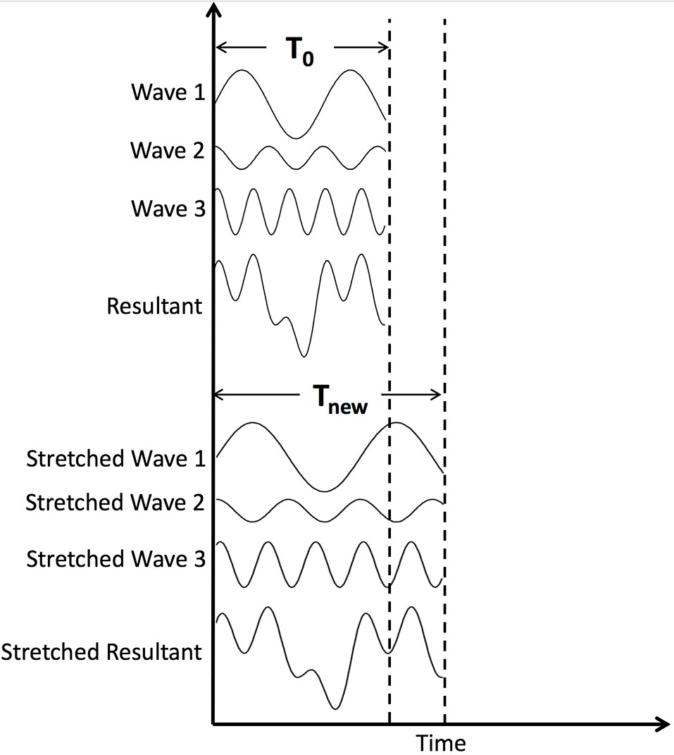
The revised age for the B–M reversal boundary has stretched the SIMPLEX timescales assigned to the two core sections, but, as before, age down the core still varies linearly with depth. Hence, it is fairly easy to estimate the new expected periods of the dominant spectral peaks. Figure 10 illustrates the logic behind this method with a hypothetical signal constructed by superposing three different waves. The original length of time corresponding to the sampled portion of the composite waveform is T0. After stretching of the timescale, this length of time becomes Tnew. Note, however, that increasing the timescale to Tnew has not changed the shape of the resultant waveform. Furthermore, since the resultant waveform is composed of simple sinusoids, the amplitudes and relative phases of the sinusoids are unaffected by this stretching.
Because the shapes of the individual sinusoids have not been affected by the stretching of the timescale, the number of wave cycles N (i.e. the number of periods) contained within the time interval for waves 1, 2, and 3 will be the same both before and after the stretching process. For instance, wave 2 in figure 10 exhibits N ≈ 3.2 periods within the space of time T0. After stretching, the number of cycles N will still be about 3.2, but those 3.2 wave cycles must now fit into the larger time interval Tnew. But the number of periods N may be calculated by dividing the original time interval T0 by the original period estimate for wave 2, which we here call P0. Thus, if we know the original period P0 for wave 2, we can estimate the new period Pnew:

Eq. (5) may also be used to estimate the new periods for the other two waves comprising the composite signal.
Here we have made an assumption that is generally not strictly correct, but which is ‘good enough’ for our purposes. We assume that the frequency of a dominant spectral peak corresponds exactly to the frequency of one of the individual waves comprising the resultant signal. Because the signal is composed of a finite number of waves, this is not really correct—an estimated peak frequency often falls ‘between’ two of the discrete frequencies in the power spectrum. Nevertheless, for a power spectrum with a reasonably large number of discrete frequencies within a finite frequency band, we expect a particular peak frequency to be quite close to one of those discrete frequencies. This means that we can also use Eq. (5) to estimate the new periods (after stretching) of the spectral peaks, provided that we know the original periods for those peaks. In the following discussion, we treat the Blackman–Tukey method of obtaining those original period estimates as a ‘black box’ and accept as a given that the original period estimates are accurate.
Confirming the results


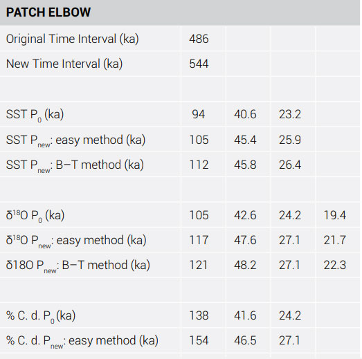
My original SIMPLEX values of P0 (obtained using my reconstructed Pacemaker data and the Blackman–Tukey method) are shown in tables 2 and 3. For instance, the middle section of table 2 lists my original periods for the three dominant RC11-120 δ18O spectral peaks. The period of the smallest spectral peak was 23.8 ka. Eq. (5) implies that the estimated value for the new (stretched) period is Pnew = (308.75 ka ÷ 273.00 ka) × 23.8 ka = 26.9 ka. This compares favourably with the new period of 27.1 ka I obtained using the Blackman–Tukey method. The agreement between these estimated periods and those obtained by the B–T method is generally poorer for the longer (~100 ka) periods (i.e. the estimated uncertainty in the new period estimate is larger for larger periods). The reason for this is given in the online appendix,43 which provides a means of estimating this uncertainty.
Unlike the SIMPLEX timescales, the ELBOW timescale for the PATCH Composite ‘core’ did not have a perfectly constant slope versus depth; the radiocarbon age of 9.4 ka (table 2 in the Pacemaker paper) remained the same both before and after stretching of the timescale, and a third anchor point (at 8.25 cm) was used in the E49-18 section of the PATCH core. Hence, this shortcut method was not strictly valid, and I did not calculate error estimates for this particular case. Nevertheless, there was still generally good agreement between periods calculated using this ‘easy’ method and the B–T method (table 4).
These comparisons were obtained using my estimates for the periods of the spectral peaks, calculated using reconstructed data. Although these results are generally in good agreement with the original published Pacemaker results, there are some discrepancies, likely due to subtle errors in the values of the reconstructed data. However, one can also use this method and the original published Pacemaker results to estimate the periods that the Pacemaker authors would have themselves obtained had they used the currently accepted age of 780 ka for the B–M reversal boundary in their calculations.
Since the earth’s inferred orbital cycles are quasi-periodic, the frequencies expected from Milankovitch theory will not be exactly the same before and after the stretching of the timescales for the cores. However, one typically expects periods of lengths ~100, 41, and 19–23 ka to result from such orbital calculations. The new results are generally in poor agreement with Milankovitch expectations. This is especially true for the new E49-18 and PATCH results (tables 3 and 4).
Power to the people!
That the original Pacemaker results are now moot has important implications for both geochronology and ‘climate change’ speculation, discussed in part 2 of this series. Due to the complicated issues involved in the ‘climate change’ debate, it is often very difficult for voters, policy makers (and even other scientists!) to verify for themselves scientific results that are relevant to the debate. This is a rare exception—laypeople without a knowledge of calculus, and even high school students, can verify these new results. I have verified for myself that the original period estimates P0 in the original Pacemaker paper are approximately correct,15 but one does not need to take my word for it in order to make a logically compelling internal critique against the Pacemaker paper. Remember that uniformitarian scientists have themselves claimed for 40 years that the original Pacemaker results were accurate and that we should believe them. For the sake of argument, one can simply accept this claim as a ‘given’. And since uniformitarians are now claiming that the age of the B–M reversal boundary is 780 ka (rather than 700 ka), the new results (which agree poorly with Milankovitch expectations) are the logical consequence of their own claims. Uniformitarians have shot themselves in the proverbial foot!
Unfortunately, this shortcut method will not work with the trials using the uppermost E49-18 data that had been omitted in the original Pacemaker analysis. However, given that the estimated age of 12 ka for the top of the E49-18 core used in those trials seems to have been obtained via little more than an educated uniformitarian guess,44 the significance of those results is somewhat in doubt, anyway.
References and notes
- Walker, M. and Lowe, J., Quaternary Science 2007: a 50-year Retrospective, J. Geological Society, London 164(6):1073–1092, 2007. Return to text.
- Oard, M.J., The astronomical theory of the Ice Age becomes more complicated, J. Creation 19(2):16–18, 2005. Return to text.
- Oard, M.J., Astronomical troubles for the astronomical hypothesis of ice ages, J. Creation 21(3):19–23, 2007. Return to text.
- Cronin, T.M., Paleoclimates: Understanding Climate Change Past and Present, Columbia University Press, New York, pp. 130–139, 2010. Return to text.
- Oard, M.J., Phase problems with the astronomical theory, J. Creation 28(2):11–13, 2014. Return to text.
- Hayes, J.D., Imbrie, J. and Shackleton, N.J., Variations in the earth’s orbit: pacemaker of the ice ages, Science 194(4270):1121–1132, 1976. Return to text.
- Muller, R.A., MacDonald, G.J. and Alvarez, W., Preface and Forward; in: Ice Ages and Astronomical Causes: Data, Spectral Analysis, and Mechanisms, Springer, Chichester, UK, pp. xiv and xvii, 2000. Return to text.
- Hebert, T.D., Paleoceanography: Orbitally Tuned Timescales; in: Steele, J.H. (Ed.), Climates and Oceans, Academic Press, Amsterdam, The Netherlands, pp. 370–377, 2010. Return to text.
- Hebert, J., The dating ‘pedigree’ of seafloor sediment core md97-2120: a case study, Creation Research Society Quarterly 51(3):152–164, 2015. Return to text.
- Hinnov, L.A. and Hilgen, F.J., Cyclostratigraphy and astrochronology; in: Gradstein, F.M., Ogg, J.G., Schmitz, M.D. and Ogg, G.M. (Eds.), The Geologic Time Scale 2012, Elsevier, Amsterdam pp. 63–83, 2012. Return to text.
- Anonymous, New Mexico Bureau of Geology and Mineral Resources: New Mexico Geochronology Research Laboratory, K/Ar and 40Ar/39Ar Methods: The 40Ar/39Ar Dating technique, 2014, geoinfo.nmt.edu/labs/argon/methods/home.html, accessed 7 May 2014. Return to text.
- Renne, P.R., Deino, A.L. Walter, R.C. et al., Intercalibration of astronomical and radioisotope time, Geology 22(9):783–786, 1994. Return to text.
- Vardiman, L., Climates Before and After the Genesis Flood, El Cajon, CA, Institute for Creation Research, p. 79, 2001. Return to text.
- Hebert, J., Revisiting an iconic argument for Milankovitch climate forcing: should the ‘Pacemaker of the ice ages’ paper be retracted? part 1, Answers Research J. 9:25–56, 2016. Return to text.
- Hebert, J., Revisiting an iconic argument for Milankovitch climate forcing: should the ‘pacemaker of the ice ages’ paper be retracted? part 2, Answers Research J. 9:131–147, 2016. Return to text.
- Hebert, J., Revisiting an iconic argument for Milankovitch climate forcing: should the ‘pacemaker of the ice ages’ paper be retracted? part 3, Answers Research J. 9:229–255, 2016. Return to text.
- Hebert, ref. 14, pp. 39–42. Return to text.
- Hebert, ref. 14, pp. 38–56. Return to text.
- Hays et al., ref. 6, p. 1123. Return to text.
- Howard, W.R. and Prell, W.L., Late Quaternary Surface Circulation of the Southern Indian Ocean and Its Relationship to Orbital Variations, Paleoceanography 7(1):79–117, 1992. Return to text.
- Shackleton, N.J. and Opdyke, N.D., Oxygen isotope and palaeomagnetic stratigraphy of Equatorial Pacific Core V28-238: oxygen isotope temperatures and ice volumes on a 105 year and 106 year scale, Quaternary Research 3:39–55, 1973. Return to text.
- Shackleton, N.J., Berger, A. and Peltier, W.R., An alternative astronomical calibration of the lower Pleistocene timescale based on ODP Site 677, Transactions of the Royal Society of Edinburgh: Earth Sciences 81(4):251–261, 1990. Return to text.
- Hilgen, F.J., Astronomical calibration of Gauss to Matuyama Sapropels in the Mediterranean and implication for the geomagnetic polarity time scale, Earth and Planetary Science Letters 104(2–4):226–244, 1991. Return to text.
- Spell, T.L. and McDougall, I., Revisions to the age of the Brunhes–Matuyama boundary and the Pleistocene geomagnetic polarity timescale, Geophysical Research Letters 19(12):1181–1184, 1992. Return to text.
- Wright, J.D., Cenozoic climate—oxygen isotope evidence; in: Steele, J.H. (Ed.), Climates and Oceans, Academic Press, Amsterdam pp. 316–227, 2010. Return to text.
- McManus, J.F., Bond, G.C. Broecker, W.S. et al., High-resolution climate records from the North Atlantic during the last interglacial, Nature 371:326–329, 1994. Return to text.
- Anonymous, Protactinium-231-thorium-230 dating, Encyclopedia Britannica, accessed 14 October 2016 at britannica.com/science/protactinium-231-thorium-230-dating. Return to text.
- Shackleton, Berger and Peltier, ref. 22, p. 258. Return to text.
- Shackleton and Opdke, ref. 21, p. 49. Return to text.
- Broecker, W.S. and van Donk, J., Insolation Changes, Ice Volumes, and the O18 Record in Deep-Sea Cores, Reviews of Geophysics and Space Physics 8(1):169–98, 1970. Return to text.
- Hebert, ref. 15, pp. 132–133. Return to text.
- Blackman, R.B. and Tukey, J.W., The Measurement of Power Spectra from the Point of View of Communications Engineering, Dover Publications, New York, 1958. Return to text.
- This peak frequency often does not agree perfectly with the frequency of one of the component waves, as the very tip of the spectral peak often is located at a frequency that falls ‘between’ two of the discrete frequencies for which values of spectral power have been calculated. However, as more and more discrete frequencies are plotted within a finite frequency band, this error will become smaller and smaller. Return to text.
- Hays, Imbrie and Shackleton, ref. 6, p. 1126. Return to text.
- Hebert, ref. 15, pp. 143–146. Return to text.
- The numbers on the vertical axes of our graphs disagree by a factor of ~2. This discrepancy appears to be the result of a normalization error on the part of the Pacemaker authors. Apparently, they forgot to multiply their spectral powers by 2 when converting from a two-sided power spectrum (negative and positive frequencies) to a one-sided power spectrum (positive frequencies only). Return to text.
- Jenkins, G.W. and Watts, D.G., Spectral Analysis and Its Applications, Holden-Day, San Francisco, CA, p. 260, 1968. Return to text.
- Berger, A. and Loutre, M.F., Insolation values for the climate of the last 10 million years, Quaternary Science Reviews 10(4):297–317, 1991. Return to text.
- The orbital data, as of 17 June 2016, were archived at: doi.pangaea.de/10.1594/PANGAEA.56040?format=html#lcol0.ds1004521. Return to text.
- Lisiecki, L.E. and Raymo, M.E., A Pliocene-Pleistocene stack of 57 globally distributed benthic δ18O records, Paleoceanography 20, PA1003, 2005, doi:10.1029/2004PA001071, MIS age estimates, lorraine-lisiecki.com/LR04_MISboundaries.txt, accessed 14 October 2016. Return to text.
- Hebert, ref. 16, pp. 241–242. Return to text.
- Woodward, J., The Ice Age: A Very Short Introduction, Oxford University Press, Oxford, United Kingdom, p. 97, 2014. Return to text.
- Broken climate pacemaker part 1 appendix. Return to text.
- Howard and Prell, ref. 20, pp. 87–91. Return to text.


Readers’ comments
Comments are automatically closed 14 days after publication.