

Journal of Creation 34(3):99–108, December 2020
Browse our latest digital issue Subscribe
Ice core oscillations and abrupt climate changes: part 1—Greenland ice cores
Secular scientists think ice cores are a major challenge to the biblical timescale. However, deep time is automatically built into their analysis of ice cores by using uniformitarian assumptions in the form of flow models and ‘tie points’. They assume the ice sheet has existed for millions of years, and that the annual layers become thinner down the Greenland ice cores. However, annual layer counting is a subjective exercise that is fitted to the assumed age of the core. The GISP2 and GRIP ice cores graphically show numerous abrupt changes in the oxygen isotope ratios, assumed to be correlated to temperature. Many other variables are correlated to the oxygen isotope ratio on the large and small scale. The Younger Dryas event is the last so-called abrupt climate change. Once ‘abrupt climate changes’ were accepted in the Greenland cores in the 1990s, they were then ‘seen’ in many other climate-related records. An isostatic correction was applied to each ice core to determine the elevation of the bedrock at the start of the Ice Age. The low elevation of the deep Greenland ice cores and the warm water surrounding Greenland result in different start times for post-Flood ice buildup.


Uniformitarian scientists and popularizers assume that ice cores absolutely disprove the short timescale of the Bible.1 However, an in-depth analysis of ice cores shows that this is not so.2 This series will delve deeper into some aspects of ice cores than found in Oard’s 2005 monograph The Frozen Record, including one question left for future research: the meaning of the many correlated variables to the isotope ratios on the large-scale and the ‘millennial’ timescale. It will also provide an explanation of the differences between the ice cores on the Greenland and Antarctic Ice Sheets within biblical earth history. Part 1 will describe Greenland ice cores, including two new ones and an explanation for the warmth before glaciation. Part 2 will describe Antarctic ice cores, especially the major difference between the ice cores on the West and East Antarctic Ice Sheets. Part 3 will provide a solution to the large-scale isotopic oscillations and the correlated variables in the ice cores, while part 4 will explain the millennial-scale variations that are different between the Greenland and Antarctic ice cores. Part 5 will explain how the anomalous early Holocene Green Sahara occurred because of the unique conditions of the Ice Age.
The uniformitarian challenge of Greenland ice cores
Six deep ice cores have been drilled on Greenland (figure 1) since the drilling of the first deep ice core,3 Camp Century, in 1966. Uniformitarian scientists claim they can actually count 110,000 ‘annual layers’ down to a depth of 2,800 m, near the bottom of the GISP2 ice core drilled near the top of the ice sheet. They believe it is as simple as counting the rings of a tree to determine its age.
However, uniformitarian scientists have assumed that the Greenland Ice Sheet has been more or less in equilibrium (the same size and thickness) for several million years, which means that their ‘annual layers’ would thin considerably down the ice cores (figure 2). Annual layers thin by the weight of the ice above and spread horizontally (figure 3). The final thickness of annual layers depends upon the amount of the ice accumulation and the amount of thinning. The annual layers are distinct near the top of the ice, but with thinning and diffusion deeper in the ice, it can be difficult to interpret them as ‘annual layers’.
Based on the assumption of deep time and equilibrium for millions of years, uniformitarian scientists have developed flow models. This determines the first guess for their presumed annual layer thicknesses that are believed to thin considerably with depth. These flow models are tuned to other events in uniformitarian earth history, called ‘tie points’, assumed to be accurately dated in other climate records. One tie point is the date of the transition from the last glacial maximum (LGM) to the early Holocene about 15,000 ka. All of these climate records, deep-sea cores, pollen cores, so-called varves, etc., already have deep time and uniformitarianism built in. Is it any wonder that uniformitarian scientists get results that confirm deep time in ice cores? This is why secular scientists and ‘old earth’ creation scientists conclude that ice cores are a fatal flaw to the biblical timescale.1 The old earth creation scholars need to analyze the ice cores in-depth and stick to biblical earth history, based on the straightforward reading of Scripture. When this is done, an alternative is discovered.


Creation-Flood model for the buildup of the Greenland Ice Sheet

The biblical model postulates that the Greenland Ice Sheet grew mostly during the Ice Age, which peaked about 500 years after the Flood in the Northern Hemisphere.4,5 The ice sheet on Greenland would continue to grow after the Ice Age maximum at the same time as the other Northern Hemisphere ice sheets melted. The continuing above-average warmth of the ocean would have grown the Greenland Ice Sheet, but the growth rate would have decreased with time. Figure 4 presents the postulated increase in the depth of the ice at Camp Century, Greenland, with time after the Flood.6 From figure 4, the Greenland Ice Sheet at Camp Century did not start building until about 200 years after the Flood and built up rapidly in 300 years to about 1,000 m thick. Camp Century then grew slowly, reaching near-equilibrium at about 3,000 years ago, or 1,500 years after the Flood. The curve shape for Camp Century likely is similar to that of the GRIP, GISP2, NGRIP, DYE-3, and NEEM ice cores, except for likely differences in the timing of the start of ice accumulation. GRIP, GISP2, and NGRIP, being near the centre of the ice sheet, likely started accumulating about 150 years after the Flood. The start of glaciation was delayed because Greenland was surrounded by warm water early in the Ice Age with early glaciation starting in the mountains (which with respect to the bedrock are mostly around Greenland’s coasts).
In both the creationist and uniformitarian models, the present-day accumulation is about 0.2 m/yr. Since the very uppermost, most recent layers have experienced almost no thinning, the uppermost annual layer thicknesses (both before and after thinning) should be about the same for both models. However, the deeper annual layers in the biblical model would be much thicker than those presumed from the uniformitarian model. With thinning due to the layers above, the average annual layer from about 175 years, the average beginning of ice buildup at the low elevations, to 500 years would be about 3 m/yr. But if we allow for thinning of the ice, the real annual layer average accumulation would be around 3–6 m/yr for those first 325 years. Part 3 will show that this is reasonable under the conditions of the Creation-Flood Ice Age. Thinning would be the greatest at the deeper depths in the ice, so the biblical annual layer thicknesses today for about 4,300 years of thinning would be close to that shown in figure 5, which is compared to the secular annual layer thickness due to deep time.7 How one views the ice sheets, either from the naturalistic or the biblical worldview, determines the results one gets upon analysis.

Uniformitarian ice core years based on assumptions
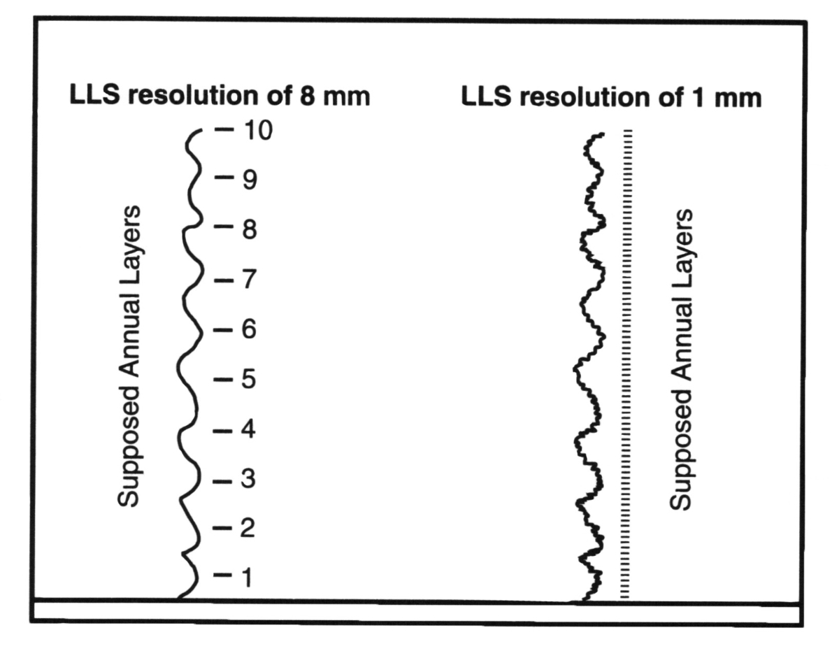
The uniformitarian scientists have essentially ‘dated’ the Greenland ice cores based on their assumptions.2,8 This was revealed when they ‘counted’ the annual layers in the GISP2 core (figure 6). The glaciologists arrived at 85,000 years at a depth of 2,800 m. Since this timescale disagreed with the timescale based on deep-sea cores and the Milankovitch mechanism, which really ‘dates’ deep-sea and ice cores (see part 2), the researchers went back and ‘re-dated’ the bottom 500 m with a higher resolution laser beam. The laser beam that detects variable dust loading went from 8 mm resolution to 1 mm resolution. Of course, with higher resolution more ‘wiggles’ were detected (figure 7). They ‘discovered’ 25,000 more wiggles, interpreted as annual layers, for an age of 110,000 years at 2,800 m—just the date they needed!9 This demonstrates one way in which deep time and the Milankovitch assumption influence observations on ice cores.
Creation scientists conclude that with an annual accumulation rate of 4–6 m/yr during the Ice Age, wiggles in each annual layer would be multiple storm or within-storm oscillations. The oxygen isotope ratios, one of the variables used in annual layer counting, can vary as much in a storm, due mainly to the warm and cold sectors, as the annual layer.10,11 Thinning and diffusion would not wipe out such oscillations with such thick annual layers. This especially shows the differences assumptions make in the analysis and results.

How do so many ice core variables correlate?
Oard’s 2005 monograph on ice cores, The Frozen Record, ended with possibilities for future research.12 One was finding how carbon dioxide, methane, various chemicals, dust, etc., measured down the ice cores, can be correlated to the oxygen isotope ratios. Many of these variables even correlate with what are believed to be millennial-scale changes. The changes are so rapid that they are called ‘abrupt climate changes’ (figure 8). Uniformitarian scientists have difficulty explaining many of these correlations. How all these variables correlate will be explained within the biblical Ice Age model for the large scale in part 3 and the small scale in part 4.

Abrupt climate changes seen in the Greenland ice cores
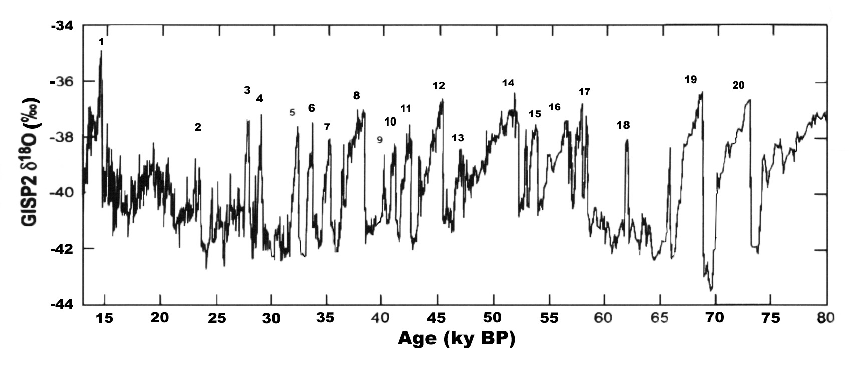
In the 1990s, a paradigm shift took place in glacial paleoclimatology.13 It was discovered from the two deep ice cores, GISP2 and GRIP, drilled 28 km (17 mi) apart at the top of the Greenland Ice Sheet (figure 1), that the oxygen isotope ratio fluctuated abruptly numerous times (figure 9).14,15 The oxygen isotope ratio is defined as: δ18O = [(18O/16O)sample – (18O/16O)standard]/ (18O/16O)standard × 1,000‰ (1) It is measured in parts per thousand or per million, and there are several standards.
These oxygen isotope fluctuations are also correlated to changes in other variables such as various chemicals (figure 8).16,17 The most important ions that determine the origins of many chemicals are sodium and calcium. Approximately 95% of sodium is of marine origin, while almost all calcium is of continental origin.16,17 High concentrations of these chemicals are correlated with low oxygen isotope ratios for stadials and vice versa for interstadials. Magnesium, potassium, chloride, and sulfate are also correlated with the oxygen isotope ratios and sodium, but nitrate and ammonium are poorly correlated.
Carbon dioxide within the air bubbles in the ice is poorly correlated to the abrupt changes in Greenland cores, but it is supposedly correlated with Heinrich events with amplitude of about 20 ppmv.18 Carbon dioxide, correlated to the oxygen isotope ratios, also rises about 80 ppmv from the last glacial maximum to the early Holocene, which is considered a mystery.19 However, the details of carbon dioxide in the Greenland and the Antarctic cores do not match well during the Ice Age. One significant problem, especially in Greenland ice cores, is that carbon dioxide can be altered by dust and in situ chemicals (e.g. sulfuric acid).20 It is also observed to increase in melt layers. An extreme case of CO2 enrichment was shown by a rise of 200 ppm in only 4 cm of core.20 Organic matter in cores can also affect not only carbon dioxide measurements, but also methane measurements.21
Oxygen isotope ratios are also correlated to the amount of dust, with low oxygen isotope ratios, or colder temperatures, generally correlated to high amounts of dust in the Greenland ice cores.22 Methane, which is generally the same between the two hemispheres, is even more highly correlated to abrupt changes than carbon dioxide (figure 10).23 It can be used to correlate between the hemispheres.

The abrupt changes in the oxygen isotope ratio were noted in the earlier deep Camp Century (figure 11) and Dye-3 (figure 12) ice cores, but little attention was paid to them. To show how uniformitarian and deep time assumptions enter the analysis in the Camp Century ice core (figure 11), figure 13 shows a plot with ‘time’ and the resulting greatly stretched out lower portion of the ice core.
It was not until the GISP2 and GRIP cores were drilled at the top of the ice sheet that the abrupt oxygen isotope changes really stood out (figures 14 and 9). The abrupt changes are also seen in the new deep ice cores, NEEM and NorthGRIP (NGRIP), drilled north-west of GISP2 and GRIP (figure 1). NEEM and NGRIP ice cores are very similar to GISP2 and GRIP.


Oxygen isotope ratios are generally correlated to temperature, but there are many other variables that can affect isotope ratios, such as the temperature and oxygen isotope ratio of the evaporating seawater, the distance of travel of the moisture, the latitude, the longitude, the proportion of the precipitation that falls in summer versus winter, the precipitation intensity, the temperature in the cloud at condensation, and the number of condensation cycles.24 For the sake of discussion, we will assume that the oxygen isotope ratios are proportional to temperature.
If one interprets these oxygen isotope fluctuations just in terms of temperature within the uniformitarian system, it would mean that in the Northern Hemisphere, or at least in the North Atlantic area, the temperatures fluctuated up to 10–20°C on a millennial timescale.15 However, it was the abrupt rate of change that has startled secular scientists. The rate of change appears to have taken from a decade25 to as short as 1 to 3 years!26 The changes lasted for about a millennium or two and then shifted back again to the original oxygen isotope value.


These fluctuations are named Dansgaard-Oescher (D-O) events after two prominent researchers. It is suggested that the average period of these D-O events is about 1,470 years,27 and there are about 25 of them (only 20 of them are shown in figure 9).28 However, some researchers think there is no certain period for D-O events and that they are random.29 There are also ‘Heinrich events’, based on what are interpreted to be six to eight episodes of ice-rafted debris (IRD) dispersed about every 7,000 to 10,000 years in North Atlantic deep-sea cores.30 They are believed to have originated from the Hudson Strait Ice Stream. D-O events do not necessarily correlate with Heinrich events.31 Melting of the Laurentide and Scandinavian Ice Sheets at regular intervals are believed to have discharged an enormous number of icebergs into the North Atlantic Ocean. The icebergs are believed to have rapidly changed the heat exchange over the oceans and cooled the atmospheric temperatures.32 What is especially perplexing is that one would expect an armada of icebergs during a warm phase, but they surprisingly occur just after extreme cooling and during the millennial-scale cold periods.33 The data on Heinrich events, of course, depends upon the ‘accurate dating’ of deep-sea cores and identifying true IRDs. The dating of deep-sea cores themselves depends upon evolution, uniformitarianism, and deep time.34
The special Younger Dryas event
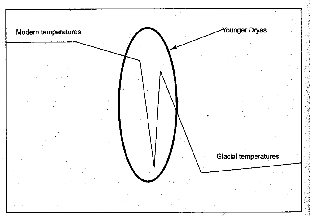
One of these abrupt climate changes that had been noticed for a long time, before the 1990s, is the Younger Dryas cold event (figure 15). It is the last cold fluctuation during deglaciation after the warm Bølling-Allerød event. The Younger Dryas is supposed to have lasted about 1,000 to 1,500 years at the very end of the ‘last’ ice age. It had a temperature drop of about 15°C relative to today35 and is dated about 11,700–12,900 years ago.
Dr Larry Vardiman, formerly of the Institute for Creation Research, believes that changing sea ice areas or an ice shelf change can produce the Younger Dryas cold event.6 Although it is possible, this hypothesis seems unlikely because the Younger Dryas is similar to all the other abrupt climate changes during the Ice Age, even near the beginning of ice buildup. There would have been no significant sea ice in the early-to-mid Ice Age because of the warm oceans. Sea ice would have increased rapidly during deglaciation since fresh water floats on salt water and freezes more easily. It is likely the sea ice covered a greater area than today by the end of the Ice Age. So, we must look for another mechanism, which will be discussed in part 4.
Abrupt climate changes suddenly seen in other climatic data sets
It is amazing that abrupt climate shifts were rarely if ever seen in other such post-Flood climate records before the GISP2 and GRIP ice cores were drilled. But once those ice cores were analyzed, the idea of catastrophic climate shifts took hold. It is interesting that researchers later ‘discovered’ them in many other climatic data sets on land and sea, for instance in deep sea cores and lake pollen data.13 They are also seen in the tropics.36,37 Sarnthein et al. state:
“Since these first discoveries from the Greenland Summit cores in the early 1990s, the record of this unexpected climatic behavior has been found in many regions, including polar ice sheets; marine sediments of the Atlantic, Pacific, and Indian Oceans; and in terrestrial lakes and bogs.”38
Drijfhout et al. support this deduction:
“Abrupt climate change is abundant in geological records, but climate models rarely have been able to simulate such events in response to realistic forcing.”39
Are we witnessing another example of the ubiquitous reinforcement syndrome, where deductions from one data set, abrupt changes, are ‘seen’ in other data sets?40

Isostatic considerations before glaciation
It is important to consider isostatic effects of the ice sheets, since these will be important in explaining the differences between the Greenland and Antarctic ice cores. The time that each Greenland ice core started accumulating ice likely determines the large-scale features of each ice core. We must first correct for isostasy to determine the bedrock elevation before the Ice Age. In general, as ice builds up, the bedrock is pushed down by the weight of the ice. The upper crust is considered elastic and the up and down motion of the bedrock is called isostasy. The amount of isostatic sinking is believed to be about 1/3 the thickness of the ice above,41 based largely on the ratio of the density of ice (~910 g m–3) to that of the asthenosphere (~3,300 g m–3).42 So, a 3,000 m thick ice sheet would compress the land about 1,000 m (figure 16). To go backwards to the beginning of ice buildup, we must raise the land by that amount. We will assume that the isostatic change is 1/3 the thickness of the ice at each core location, although isostatic effects are likely caused by more regional ice thicknesses and not point thicknesses. The range of elevation recovery for the Greenland ice core locations ranged from 463–1,110 m.
Table 1. Calculation of the estimated bedrock elevations of Greenland ice core locations before the Ice Age based on an isostatic correction of 1/3 the thickness of the ice
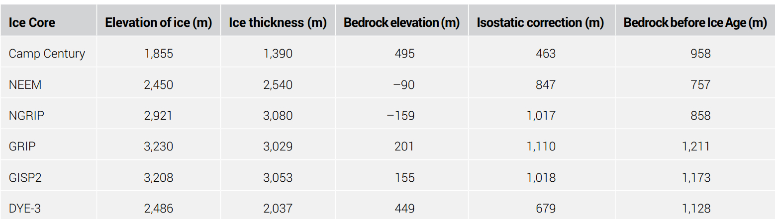
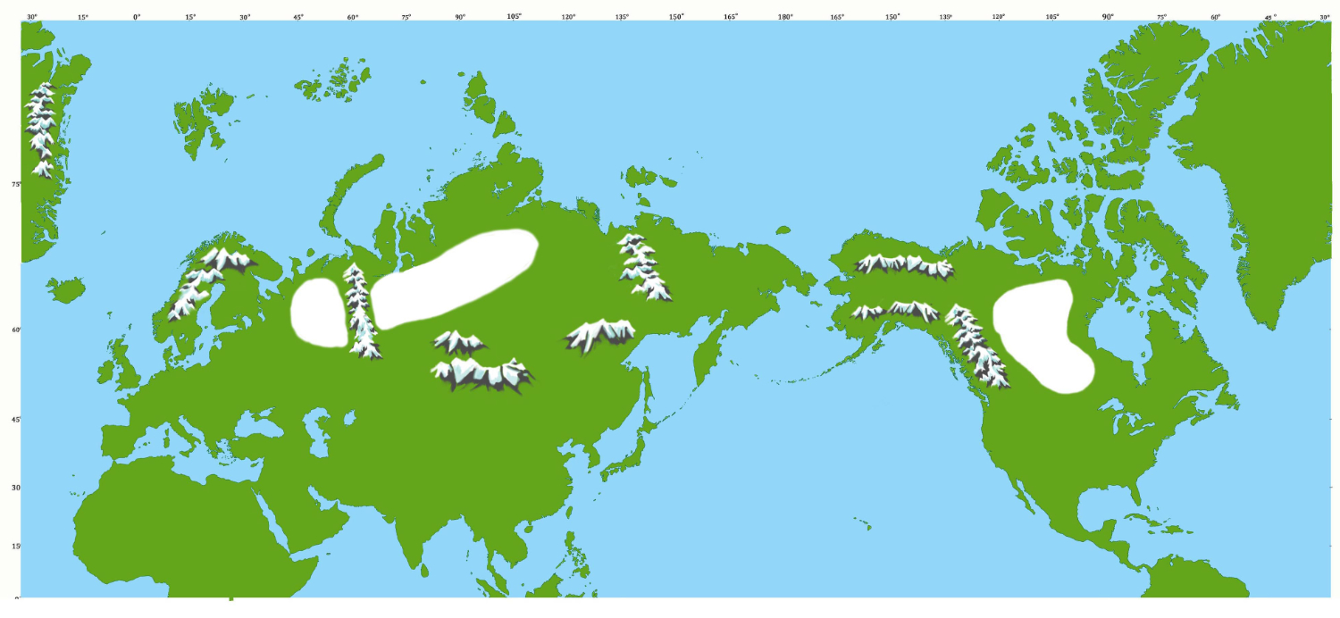
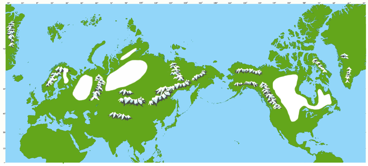
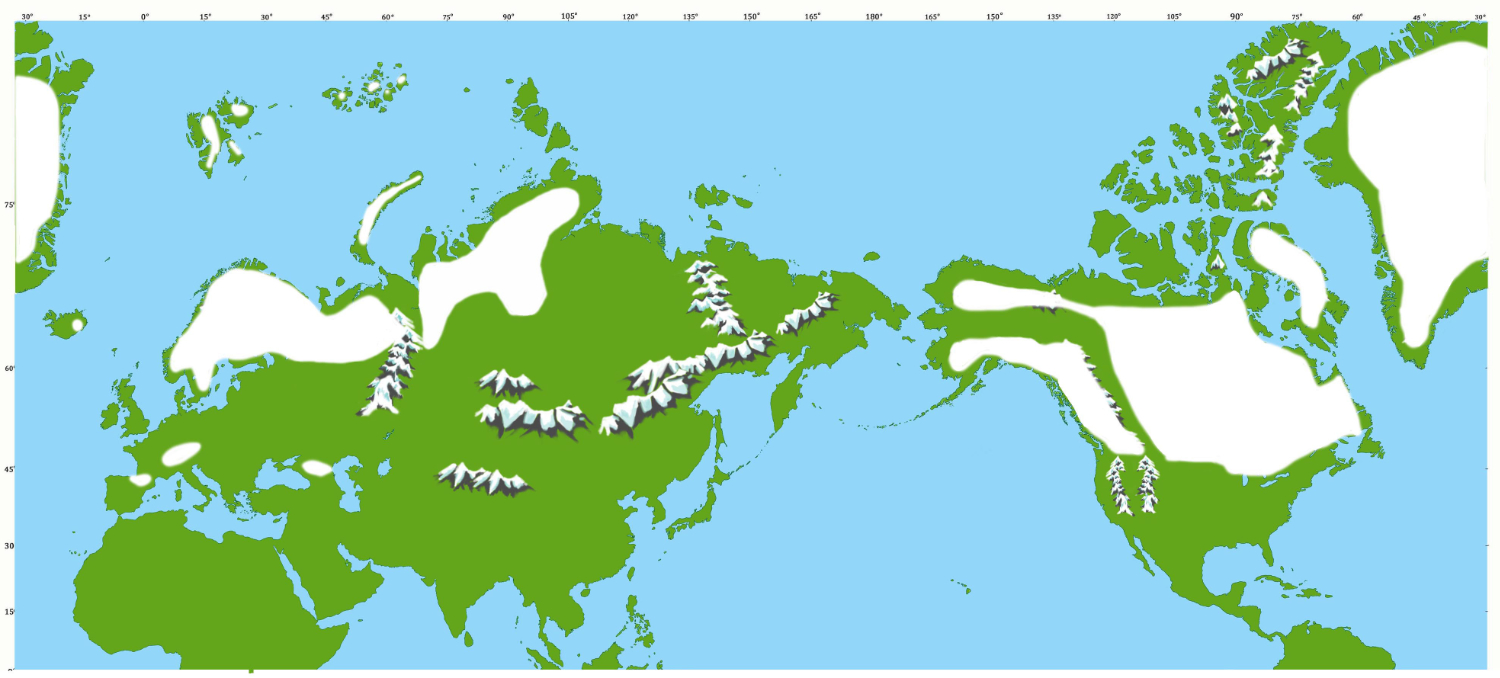
Table 1 presents the current altitude, ice thickness, present bedrock elevation, isostatic correction, and the height of the bedrock at the beginning of the Ice Age. The lowlands were in general around 1,000 m above sea level (asl) at the beginning. The ice would delay in these lowland locations of Greenland because the snow and ice built up first in the mountains before it spread to the lowlands of Greenland (figures 17–19). The warm water surrounding Greenland held off the ice in the lowlands for a while. Each ice core likely started accumulating ice at different times between 100–200 years. It is likely GISP 2 and GRIP glaciated first since they are far from the warm ocean, which is also why the Ice Age ice is thicker there. Camp Century, on the other hand, was close to the warm ocean water and would glaciate later, resulting in a thinner Ice Age portion of the ice core (compare figures 11 and 14).
Summary
The properties of Greenland ice cores are summarized showing the large-scale and small-scale abrupt change in the oxygen isotope ratios. Deep time is automatically built into Greenland ice cores by assuming the ice sheet has been in equilibrium for millions of years. This assumption determines the number of annual layers, measured at the top of the ice sheet, that thin with depth. Annual layer counting is shown to be a subjective exercise, assuming deep time, and the astronomical or Milankovitch theory of the ice ages. Many other variables, such as calcium, sodium, carbon dioxide, methane, and dust, are correlated to the oxygen isotope ratio. The abrupt changes are assumed to be millennial-scale fluctuations in temperature that change abruptly, in years to a few decades. After the discovery of ‘abrupt climate changes’ in GISP2 and GRIP, they were ‘discovered’ in many other climate-related data sets. Isostatic rebound was employed to find the elevation of the ice core locations at the beginning of the Ice Age, which will be important for determining average ice sheet growth and the differences between the Greenland and Antarctic ice cores in part 3.
References and notes
- Seely, P.H., The GISP2 ice core: ultimate proof that Noah’s Flood was not global, Perspectives on Science and Christian Faith 55(4):252–260, 2003. Return to text.
- Oard, M.J., The Frozen Record: Examining the Ice Core History of the Greenland and Antarctic Ice Sheets, Institute for Creation Research, Dallas, TX, 2005 (available from ICR by print on demand). Return to text.
- The six deep cores are Camp Century, Dye-3, GRIP, GISP2, NGRIP, and NEEM. Other cores are either shallow, such as Crete and Milcent, or drilled in the mountains, such as Renland. Return to text.
- Oard, M.J., Frozen in Time: Woolly mammoths, the Ice Age, and the biblical key to their secrets, Master Books, Green Forest, AR, 2004. Return to text.
- Oard, M.J., The Great Ice Age: Evidence from the Flood for its quick formation and melting, Awesome Science Media, Richfield, WA, 2013. Return to text.
- Vardiman, L., Rapid changes in oxygen isotope content of ice cores caused by fractionation and trajectory dispersion near the edge of an ice shelf, J. Creation 11(1):52–60, 1997. Return to text.
- De Angelis, M., Steffensen, J.P., Legrand, M., Clausen, H., and Hammer, C., Primary aerosol (see salt and soil dust) deposited in Greenland ice during the last climatic cycle: comparison with East Antarctic records, J. Geophysical Research 102(C12):26681–26698, 1997. Return to text.
- Oard, M.J., Do Greenland ice cores show over one hundred thousand years of annual layers? J. Creation 15(3):39–42, 2001. Return to text.
- Meese, D.A. Gow, A.J., Alley, R.B., Zielinski, G.A., Grootes, P.M., Ram, M, Taylor, K.C., Mayewski, P.A., and Bolzan, J.F., The Greenland Ice Sheet Project 2 depth-age scale: methods and results, J. Geophysical Research 102(C12):26411–26423, 1997. Return to text.
- Epstein, S. and Sharp, R.P., Oxygen-isotope variations in the Malaspina and Saskatchewan glaciers, J. Geology 67:88–102, 1959. Return to text.
- Gedzelman, S.D. and Lawrence, J.R., The isotopic composition of cyclonic precipitation, J. Applied Meteorology 21:1385–1404, 1982. Return to text.
- Oard, ref. 2, pp. 141–145. Return to text.
- Oard, M.J., A tale of two Greenland ice cores, J. Creation 9(2):135–136, 1995. Return to text.
- Oard, ref. 2, pp. 123–135. Return to text.
- Oard, M.J., Wild ice-core interpretations by uniformitarian scientists, J. Creation 16(1):45–47, 2002. Return to text.
- Mayewski, P.A. et al., Changes in atmospheric circulation and ocean ice cover of the North Atlantic during the last 41,000 years, Science 263:1747–1751, 1994. Return to text.
- Mayeweski, P.A., Meeker, L.D., Twickler, M.S., Whitlow, S., Yang, Q., Lyons, W.B., and Prentice, M., Major features and forcing of high-latitude northern hemisphere atmospheric circulation using a 110,000-year-long glaciochemical series, J. Geophysical Research 102(C12):26345–26366, 1997. Return to text.
- Stauffer, B., Blunier, T., Dällenbach, A., Indermühle, A., Schwander, J., Stocker, T.F., Tschumi, J., Chappellaz, J., Raynaud, D., Hammer, C.U., and Clausen, H.B., Atmospheric CO2 concentration and millennial-scale climate change during the last glacial period, Nature 392:59–62, 1998. Return to text.
- Beeman, J.C., Gest, L., Parrenin, F., Raynaud, D., Fudge, T.J., Buizert, C., and Brook, E.J., Antarctic temperature and CO2: near-synchrony yet variable phasing during the last glaciation, Climate of the Past 15:913–925, 2019. Return to text.
- Smith, H.J., Wahlen, M., Mastrioianni, D., Taylor, K., and Mayewski, P., The CO2 concentration of air trapped in Greenland Ice Sheet Project 2 ice formed during periods of rapid climate change, J. Geophysical Research 102(C12):26577–26582, 1997. Return to text.
- D’Andrilli, J., Foreman, C.M., Sigl, M., Priscu, J.C., and McDonnell, J.R., A 21,000-year record of fluorescent organic matter markers in the WAIS Divide ice core, Climate of the Past 13:533–544, 2017. Return to text.
- Ram, M. and Koenig, G., Continuous dust concentration profile of pre-Holocene ice from the Greenland Ice Sheet Project 2 ice core: dust stadials, interstadials, and the Eemian, J. Geophysical Research 102(C12):26641–26648, 1997. Return to text.
- Stowasser, C., Buizert, C., Gkinis, V., Chappellaz, J., Schüpbach, S., Bigler, M., Faïn, X., Sperlich, P., Baumgartner, M., Schilt, A., and Blunier, T., Continuous measurements of methane mixing ratios from ice cores, Atmospheric Measurement Techniques 5:999–1013, 2012. Return to text.
- Oard, ref. 2, pp. 147–158. Return to text.
- Pausata, F.S.R., Legrande, A.N., and Roberts, W.H.G., How will sea ice loss affect the Greenland Ice Sheet? EOS Transactions of the American Geophysical Union 97(9):10, 2016. Return to text.
- Hammer, C., Mayewski, P.A., Peel, D., and Stuiver, M., Preface to special volume on two Greenland ice cores, J. Geophysical Research 102(C12):26315–26316, 1997. Return to text.
- Schulz, M., On the 1470-year pacing of Dansgaard-Oeschger warm events, Paleoceanography 17(4):1–10, 2002. Return to text.
- Capron, E., Landais, A., Chappellaz, J., Buiron, D., Fisher, H., Johnsen, S.J., Jouzel, J., Leuenberger, M., Masson-Delmotte, V., and Stocker, T.F., A global picture of the first abrupt climatic event occurring during the last glacial inception, Geophysical Research Letters 39(L15703):1–8, 2012. Return to text.
- Ditlevsen, P.D., Andersen, K.K., and Svensson, A., The DO-climate events are probably noise induced: statistical investigation of the claimed 1470 years cycle, Climate of the Past 3:129–134, 2007. Return to text.
- Hesse, A. and Khodabakhsh, S., Anatomy of Labrador Sea Heinrich layers, Marine Geology 380:44–66, 2016. Return to text.
- Andrews, J.T. and Voelker, A.H.L., ‘Heinrich events’ (& sediments): a history of terminology and recommendations for future usage, Quaternary Science Reviews 187:31–40, 2018. Return to text.
- Fronval, T., Jansen, E., Bloemendal, J., and Johnsen, S., Oceanic evidence for coherent fluctuations in Fennoscandian and Laurentide Ice Sheets on millennium timescales, Nature 374:443–446, 1995. Return to text.
- Strikis, N.M., et al., South American monsoon response to iceberg discharge in the North Atlantic, Proceedings of the National Academy of Science (PNAS) 115(15):3788–3793, 2018. Return to text.
- Oard, M.J., The Deep Time Deception: Examining the case for millions of years, Creation Book Publishers, Powder Springs, GA, 2019. Return to text.
- Severinghaus, J.P., Sowers, T., Brook, E.J., Alley, R.B., and Bender, M.L., Timing of abrupt climate change at the end of the Younger Dryas interval from thermally fractionated gases in polar ice, Nature 391:141–146, 1998. Return to text.
- Pahnke, K., Zahn, R., Elderfield, H., and Schulz, M., 340,000-year centennial-scale marine record of Southern Hemisphere climatic oscillations, Science 301:948–952, 2003. Return to text.
- Rashid, H., Understanding the extent and causes of abrupt climate change, EOS Transactions of the American Geophysical Union 90(42):376, 2009. Return to text.
- Sarnthein et al., Exploring Late Pleistocene climate variations, EOS Transactions of the American Geophysical Union 81(51):625, 2000. Return to text.
- Dfijfhout, S., Gleeson, E., Dijkstra, H.A., and Livina, V., Spontaneous abrupt climate change due to an atmospheric blocking—sea-ice—ocean feedback in an unforced climate model simulation, PNAS 110(48):19713–19718, 2013; p. 19713. Return to text.
- Oard, M.J., Ancient Ice Ages or Gigantic Submarine Landslides? Creation Research Society Books, Chino Valley, AZ, pp. 11–13, 1997. Return to text.
- Bamber, J.L., Layberry, R.L., and Gogineni, S.P., A new ice thickness and bed set for the Greenland Ice Sheet 1. Measurements, data reduction, and errors, J. Geophysical Research 106 (D4):33773–33780, 2001. Return to text.
- Le Meur, E. and Huybrechts, P., A comparison of different ways of dealing with isostasy: examples from modelling the Antarctic Ice Sheet during the last glacial cycle, Annals of Glaciology 23:309–317, 1996. Return to text.
- De Angelis, M., Steffensen, J.P., Legrand, M., Clausen, H., and Hammer, C., Primary aerosol (sea salt and soil dust) deposited in Greenland ice during the last climatic cycle: comparison with East Antarctic records, J. Geophysical Research 102(C12):26681–26698, 1997. Return to text.
- Vardiman, L., Climates Before and After the Genesis Flood: Numerical models and their implications, Institute for Creation Research, Dallas, TX, 2001. Return to text.

Readers’ comments
Comments are automatically closed 14 days after publication.