

Journal of Creation 29(1):72–79, April 2015
Browse our latest digital issue Subscribe
Modelling biblical human population growth
The Bible presents several historical scenarios in which the human population grew from very small numbers. These include the initial populating of the world starting with Adam and Eve and the repopulating of the earth from three founding couples after Noah’s Flood. There were also multiple small-scale duplications of these events within the many post-Babel populations, including the growth of the Hebrew nation from Jacob and his twelve sons. Most modern commentators on the subject of biblical demographics have assumed a smooth increase in the population over time, but small populations do not tend to grow in an algebraic manner. We wanted to analyze many different biblical scenarios, so we created a population modelling program in the C# programming language that could handle multiple variables like age of maturation, minimum child spacing, and age of menopause, as well as probabilities like polygamy, twinning rates, and a variable risk of death according to age. We were able to demonstrate that the current world population and the size of the Exodus population are easy to account for under most parameter settings. The size of the antediluvian and Babel populations, however, remain unknown.
Multiple authors have written briefly about the mathematical feasibility of the demographic claims in the Bible. Most have concluded there is no biblical paradox but most have only cursorily dealt with the issues involved. Despite occasional claims from skeptics,1 it is entirely possible to obtain significant numbers of people in short amounts of time.2
This includes reaching a world population of over 7 billion people in only ~4,500 years since the Flood.3 Morris was the earliest reference we could find for someone who attempted an algebraic solution.4 He attempted to account for generation time, family size, and longevity in his calculations but this was prior to the invention of the personal computer and he simply could not track as many variables as is possible today. Later commentators have tended to use a simple algebraic approach (see the exponential growth formula below) to answer these questions as well.
Population growth depends on a combination of birth rate and death rate and is affected by the carrying capacity of the environment. Humans, unlike other species, have the ability and intelligence to grow beyond what would otherwise be the environmental carrying capacity, witnessed by the dramatic growth of the world population in recent decades.
While we do not know what environmental challenges the antediluvian and immediate post-diluvian populations faced, human populations have the ability to grow quite quickly. Based on numerous examples from recent history, we expect the early post-Creation and post-Flood generations would have experienced a rapid population increase, under a wide range of potential conditions, but what rate of growth is reasonable?
The standard exponential model of population growth is as follows:
where N = the population size at time t, N0 is the population size at time 0, and k = the growth rate. Importantly, this formula should only be applied to large populations. While it is true that the human population only needed to average a 0.464% growth rate (k) to go from 6 (N0) to 7 billion (N) people in the c. 4,500 years (t) since the Flood, the growth of small populations is stochastic by nature. One reason for this is the fact that random births and deaths have a much greater effect in a population of, for example, 10 individuals than they do in a population of 10,000 individuals.
Another reason is the unpredictable availability of members of the opposite sex in very small populations. Consider a biblical model starting with Adam and Eve. The population size at 100 years could be drastically different if they had children in the order boy-girl-boy-girl-boy-girl versus a scenario where they had a series of boys (or a series of girls) in the early years. Thus, it is impossible to predict or accurately model the growth of small populations with the exponential growth formula.
Modern genetic data indicate the human population has exploded over the past several thousand years.5 But that is only considering the size of the population. In fact, excess population has had a significant factor throughout much of world history. For example, various Greek colonies were founded across the Mediterranean and Black Sea regions by young people looking for space.
Likewise, the invasions of the Germanic tribes into Roman Europe in the waning years of that empire were driven in part by population expansion. And the Viking invasions across Europe several centuries later were propelled by that population’s ability to raise more children than the culture could provide space for.6 Throughout recorded human history, the rate of population growth has often been great enough to put extreme pressure on land ownership and the control of resources, sometimes leading to mass migration, and often sparking wars.
One might ask, “Given the high reproductive capacity of people, why has the population grown so slowly?” The answer is probably that most people ever born probably died of warfare (often fuelled by population excess), starvation (due to war or weather), or disease before they reached their full reproductive potential. These factors are very much dependent on population density, however, and so should have less impact when a population is small and growing.
Biblically, the entire human race descends from just two people, Adam and Eve. Growing to unknown numbers over the first one and a half millennia, the population then went through an extreme but short bottleneck when only eight people survived Noah’s Flood. From the three sons of Noah (and their three wives), the population grew again to unknown numbers before being subdivided at the Tower of Babel, whereupon each of the resulting subpopulations followed an independent, and complex, growth trajectory.
Those three demographic expansion events need to be addressed mathematically to see if they comport to reality. An additional population expansion mentioned in the Bible is that of the Israelites. Only a few centuries after Jacob, his twelve sons, and their children moved to Egypt,7 several million Hebrews left at the Exodus. Some argue for a ‘short’ sojourn of 215 years, while others argue for a ‘long’ sojourn of 430 years. This is a long-standing textual debate that also influences the date of creation.8
The large size of the Israelite population at the Exodus has been used as a critique of the short sojourn hypothesis.9 Is this a valid critique? Can 12 adult couples produce several million people in just 215 years?

We understand that it is possible to get a large population in a short amount of time, but do all scenarios lead to such population growth? And how likely is it that the sparse biblical data actually match the historical record? We wanted to explore the demographic possibilities within each of these major biblical scenarios. To that end, we wrote a computer program that tracked as many factors as possible, including age of maturation, minimum child spacing, age of menopause, rates of polygamy, twinning rates, and a death probability based on actuarial tables.
We also wanted our model to be flexible enough to examine post-Creation, post-Flood, and both the long and short Egyptian sojourn scenarios. Historically, most population models use discrete cohorts, where each generation is treated as a discrete set and removed from the population model after reproducing. This is sufficient for species with an annual life-death cycle, and works well enough for long-lived species with large population sizes, but it is not sufficient for the biblical scenarios we wanted to model. Instead, we tracked each individual separately and used probability distributions to determine their survival, marriage, and number of children.
This allows for more realistic scenarios where members of different generations may mate.
Methods
We constructed a population tracking program in the C# programming language that can be used for a wide range of scenarios, including both large and small populations (up to the limits of available computer memory).10 For each scenario modelled, we set minimum childbearing ages (CBA) for females and males. This was the age at which children were entered into the marriage pool. We also set a maximum CBA for females.
We set the probability of a man getting married after passing the minimum CBA at 50% per year (6.7% per 1/10 year) if at least one lady was available. Once married, we assigned an initial annual pregnancy probability of 0.88. Children were born to each married couple with a minimum child spacing until the female reached the maximum childbearing age.
In order to approximate the risk of death, we incorporated the 2009 US actuarial tables11 into our model. This should be sufficient for asking how the modern human population could grow from three founding couples but we modified the curve in some model runs to better reflect the biblical data. For example, since the modern life expectancy of 75-80 years is approximately 1/12th the typical lifespan of 900 years before the Flood, we multiplied the age for death probabilities at each stage by 12 while modelling the antediluvian population.
The Maximum Age parameter sets the age at which the probability of dying that year reaches 1. Due to the exponentially increasing probability of death as age increases, only a tiny fraction of the population came to within 5% of the set maximum in any model run, as with real human populations. The actuarial table we used for our model (with a maximum age of 120) is based on modern populations, in which typically the oldest person known to be alive anywhere on earth is 114 or 115.
Although people in ancient populations probably suffered more early death due to disease and injury, while the elderly who avoided those risks lived longer than modern humans (at least through the Exodus), we are assuming the probability of death curve was similar then to now. In all post-Flood models reported here, we set the maximum age to 120, unless otherwise specified.
On top of the standard mortality tables, we added an extra factor to account for an increased risk of maternal mortality prior to the advent of modern medicine. Since childbirth has historically been the greatest mortality risk for women of childbearing age, we allowed a set risk of maternal mortality for each birth (double for twins), and we could modify the value as needed. We assumed that the child also died if the mother died. This parameter has some overlap with both the minimum child spacing setting and the actuarial tables, but it allowed us increased flexibility to explore various scenarios.

Since we are dealing with ancient societies, we included the ability to model the effects of polygamy (more specifically, polygyny). There exist quite a large number of possibilities, so we settled on what seemed like a reasonable scenario and built flexibility into the program so we could explore alternate scenarios if necessary.
When the most generic model of polygamy was enabled, 1% of men with one wife were allowed first pick of the available females in the population. Men with two or more wives had a 5% probability of adding more. We set the maximum number of wives to 5. The remaining females were allowed to marry the remaining males at random. As always, any unmarried individuals were held over for the next round. Females who passed the maximum CBA while available were moved to the “widows” list.
When individuals were born into the population, they were assigned a birth date in tenths of years.12 This was done as a compromise. Annual increments led to stochastic outputs or strong ‘cohort’ effects where multiple children were reaching maturation and marrying at the same time, creating distinct pulses of population growth through childbirth, especially in the early years of population growth. On the other hand, dividing up years into 365 increments was computational overkill.
Model assumptions
Even though we attempted to be as comprehensive as possible, there were several areas where we simply had to make assumptions. For example, we assume a rate of twinning of 1 in 89 births. This ratio changes over time and across cultures13 but since it is less than 2% of all births, it should have but a small effect on population growth.
Likewise, there is no available data for ancient maternal mortality when carrying twins, and ancient mortality rates should be higher than today, so we simply doubled the set maternal mortality rate for twins. We did not even consider triplets, for they are several orders of magnitude more rare and the maternal death rates in these cases were extreme for times more than 100 years ago.
We allowed for remarriage after the death of a spouse, but only as long as the living partner was below the CBA cutoff. Even though males could theoretically father children if they were above their CBA, we simplified things by not allowing them to remarry if older than that. Once married, couples stayed married until death.
See table 1 for the adjustable parameter list.
Results
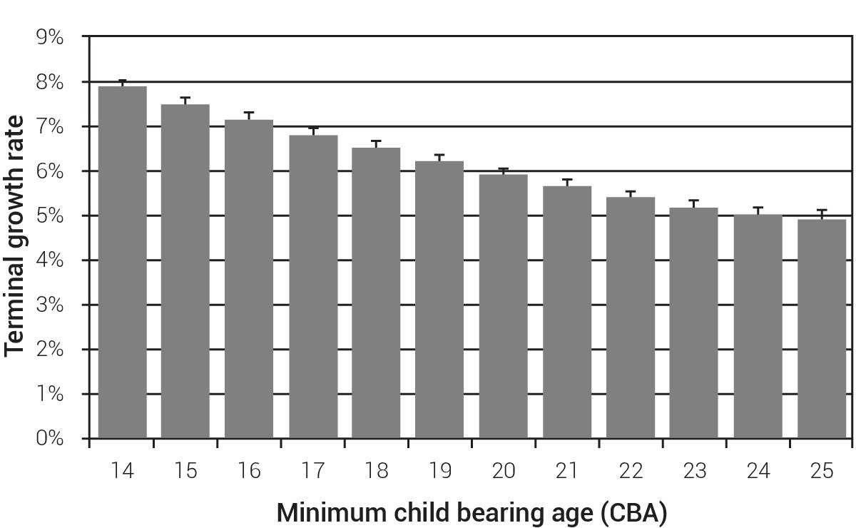
Model validation— Figures 1, 2 and 3 show summary results of a simple model of population growth. Minimum child spacing was set to 1 year. Minimum CBA ranged between 14 and 25. Maximum CBA was set to 45. Maximum age was set to 120, but this parameter had little effect on the final results because very few people lived to anywhere near the maximum age. Results are the average of 1,000 model runs for each setting of CBA. Figure 1 shows the terminal growth rates (the slope of the line from each graph of population size versus time), calculated from the final order of magnitude of population growth (approximately the final 20%) of each model run.

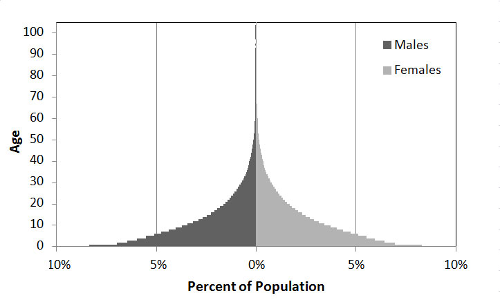
Figure 2 shows the population structure of a model run with minimum CBA set to 14. The thin, tall peak in the chart is due to a high maximum potential age (a very few people simply lived a long time). The shape of the distribution is similar to that of a ‘young’ population like that of modern Nigeria.14
When minimum CBA increases, there are proportionally fewer young individuals in the population and the pyramid has a narrower base (data not shown). When minimum CBA is set to very high values, we noticed a ‘cohort’ effect, where the delay in reproduction produced several waves of population growth as multiple individuals reach reproductive age simultaneously.15 This is similar to the ‘baby boom’ that occurred in Western countries after World War II. These waves were due to the fact that we started with N couples already at reproductive age but with no children.
All modelled populations took several decades to settle down into a regular, algebraic growth phase. Most of the variability occurred when the population size was less than 100 individuals and almost all variability was evened out by the time 1,000 individuals were alive.
Figure 3 shows the percent survivorship curve for a modelled population with minimum CBA set to 14.
From the Flood to the modern population
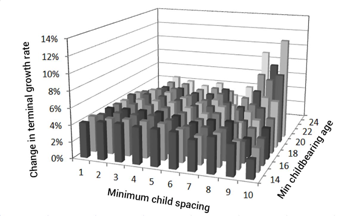
Figure 4 displays the results of a multi-parameter model run (minimum child spacing versus minimum CBA), using modern (USA 2009) actuarial data and a post-Flood-like scenario with three founding couples. We allowed the minimum child spacing to range from 1 to 10 years and the minimum childbearing age to range from 14 to 25 years. In almost all scenarios where the population did not go extinct, the critical level of 0.464% (the rate required by the exponential model of population growth to reach seven billion people in 4,500 years from three founding couples, see above) increase per year was reached. In other words, it is trivial to obtain the current world population from three founding couples in four and a half millennia.
Impact of polygamy
In Figure 5 we show the effect of polygamy (polygyny). A small percentage of men were allowed up to a maximum of five wives (details in Methods). On average, most model runs experienced a boost of approximately 4% over baseline (i.e. they were growing at 104% the rate of a non-polygamous model with the same parameter settings).
Near the edge of population survivability, polygyny enabled some populations to experience more growth, on average, due to the fact that unwed women were more rare. In other model runs (data not shown) we increased the polygamy rate up to 10%. At these extreme values, there was a much stronger effect at the margins of survivability, but this levelled off at higher growth rates. For most parameter settings, the net effect was not more than an additional 1% increase over baseline.
The impact of very old people having children
By varying the maximum age of childbearing, it is possible to illustrate the potential impact of very old women having children. Figure 6 shows the terminal growth rates of multiple model runs. Each has a minimum CBA of 20. Maximum CBA varied from 40 to 100 in 5-year increments and the minimum spacing between children varied between 1, 2, or 3 years.
Children born into smaller populations have a greater percentage impact on the future population than children born into larger populations. Therefore, the impact of increasing the years of childbearing has a diminishing effect. Here, children born when a woman was 100 years old entered a population 59, 27, and 17 times larger, respectively, for the three values of minimum child spacing, than a child born when that same woman was 40.
From the Flood to the Tower of Babel
The date of the Tower of Babel event is unknown. From context, it appears the timing has something to do with a man named Peleg, whose name means ‘division’ (Gen 10:25).16 He was born c. 101 years after the Flood and lived until c. 340 years after the Flood (Gen 11).17
If the division of people occurred only 100 years after the Flood, there would not be many people in the world. However, the data behind the growth rates calculated in figure 4 indicate that under some scenarios it is possible to obtain a population size greater than 1,000 individuals in that much time. This occurred at all settings of minimum CBA with a minimum child spacing of 1 year, or with small minimum CBA and a minimum child spacing of 2 or 3 years. It is also possible to arrive at over 10,000 individuals with a minimum child spacing of 1 year and a minimum CBA ≤ 17, and up to 40,000 individuals with a minimum CBA of 14, although these are not likely scenarios.
After 340 years, it is trivial to have 1,000 individuals in the population and most parameter settings produce population sizes many orders of magnitude greater than that. How many people were in existence when the population was divided? Sadly, one cannot determine the number from numerical analyses like these.
The Sojourn
According to Exodus 12:37-38, there were 600,000 Hebrew men in the Exodus population. Numbers 1:46 gives a more precise 603,550 men aged 20 and up. There are several ways to estimate the Exodus population size. If one assumes an equal number of females and more children than adults at the Exodus, a figure of 2.7 million is a good approximation. Starting with 12 founding couples, it was possible to reach 2.7 million people within the 215-year ‘short’ sojourn model, but only under certain, favourable parameter settings (figure 7).

In the 430-year ‘long’ sojourn model, reaching a population size of 2.7 million was trivial (figure 8). Of course, the final population sizes we are reporting here are unrealistic. Environmental restraints would take over long before these extreme population sizes were reached.
The antediluvian population size
We modelled various scenarios that started with a single founding couple. As before, it was simple to obtain significant numbers in a short amount of time. However, we know very little about the age of maturation (minimum CBA), minimum or average child spacing, etc., of antediluvian women.
Therefore, there are too many unknown variables and there is no way to estimate the antediluvian population size. It could have been in the billions. Or it could have been a few thousand. We cannot know.
Discussion
Using realistic demographic parameters, all modelled populations experienced rapid growth, on average. It was entirely possible to drive a population to extinction, however. As the average number of children per female approached the ‘replacement value’, more simulation samples resulted in extinction. When the minimum CBA and child spacing was such that women could have more than two children only by bearing twins, all samples went extinct.
The exact replacement value depends on many factors. Essentially, it is the number of children each female must have in order to guarantee that at least one female child reaches adulthood, on average. The number is often cited as ‘2.1’, but it is less than that in Western cultures and often much greater than that in developing countries.18 We included parameter settings that led to extinction in figures 4 and 5 to illustrate this.
There are two main factors that influence population growth the most: minimum CBA and minimum child spacing. This makes sense in that a population will grow most quickly when people marry young and have children close together. This also means, however, that the maximum CBA is far less relevant. Furthermore, since the people who reproduce earliest will have a higher percent representation in the future population, genetics should be driving all populations towards faster reproduction, by default.

Early maturation is thus a mathematical certainty, given a population with individuals that have a range of maturation ages. This alone could explain the population-wide drop-off in lifespan after the Flood. While it is true that individual mutation count should increase over time, contributing to a decline in lifespan,19 it is also true that the ones who reproduce the fastest will outnumber those who do not. In the end, maximum lifespan does not matter.
This comes into sharp focus when considering modern cultures. For many reasons, people in wealthier ‘First World’ nations are tending to have fewer children, farther apart, and with a delayed start of childbearing. And, while China and India have huge populations, their growth is levelling off, while the population of Africa is still increasing rapidly. Life expectancy is generally higher in the slowest-growing populations.
It is not necessary to model the great ages of the biblical Patriarchs, or the fact that their ages decreased over time, because children born to these people late in life are almost irrelevant as far as their impact on future population growth is concerned. The future impact on the population size caused by the birth of any specific individual is simply the inverse of the population size at that time.
In fact, the relative individual impact on the future population size of any two people is simply the ratio of inverse population sizes when each person was born, which can be reduced to a simple ratio of the relative times when they were born:
The only caveat is that people who lived a long time may not have matured as young as modern people, so the minimum CBA might come into play to a greater degree than we illustrate here. Yet, the average generation span for the first seven generations born after the Flood is 31.4 years, and there is no reason to suspect these are all oldest children.20 Interestingly, the modern average human generation time is approximately 30 years.21
This brings up another interesting point; kingship has historically been conferred on the eldest sons. Thus, one might expect a long line of kings to experience more generations on average per century than the rest of the population.
Thus, when Jacob met Pharaoh, he asked him how old he was, as if he was surprised to have met such an old man (Gen 47:8). Jacob was but 12 generations removed from Noah and was the grandson of Abraham, who had met another Pharaoh approximately 200 years earlier. How many generations after the Flood was the Pharaoh of Jacob’s day, and how many generations was he removed from the Pharaoh who knew Abraham two centuries prior?
The subject of how many generations removed were the modelled people from the starting ancestors is fascinating.
We included this calculation for the sake of curiosity. In each run, there were always people with very long lines going back to the founding couple (essentially equal to the length of run/minimum CBA) and at the same time people with very short lines in their family tree (due to the fact that very old men could still father children with younger wives). There are modern analogues to the Abraham-Pharaoh scenario,22 so this should really be no surprise.

Concerning the Egyptian sojourn, we started with 12 couples with no children, but Gen 46:27 indicates that Jacob’s sons had already started reproducing before he moved to Egypt. In other words, the clock started before they arrived in Egypt and the 215-year sojourn is a minimum figure. Adding more individuals to the starting population size makes it easier to arrive at the required Exodus population size then we report here.
Also, Jacob brought household servants with him to Egypt (Gen 12:16, Gen 14:14, and cf Gen 46:1 “all that he had”), who might have occasionally married into the family. This is especially true of the women, but the male servants were also circumcised (Gen 17:13), meaning they were at least tangentially part of the Covenant.
Could long-standing, multigenerational, faithful, God-fearing, male family servants have married into the family as time progressed? This is likely, especially since many of them would eventually have Jacob as an ancestor, for obvious reasons.
In conclusion, it is relatively easy to explain the modern world population, starting with the six Flood survivors, in c. 4,500 years. The number of people alive at the Tower of Babel event is more difficult to determine, but could easily have been in the thousands, or even tens of thousands, under certain conditions.
The long/short sojourn debate cannot be answered with demographic data, but there is no reason to reject the short sojourn from numerical data alone. And, it is impossible to estimate the number of people alive at the Flood, for we simply do not have the necessary demographic data.
References and notes
- E.g., Repopulation after the Flood, talkorigins.org/origins/postmonth/may04.html. Return to text.
- Morris, H., How Populations Grow, undated; icr.org/article/3589. Return to text.
- Batten, D., Where are all the people? Creation 23(3):52–55, 2001; creation.com/people. Return to text.
- Morris, H.M., World population and Bible chronology, CRSQ 3(3):7–10, 1966; creationresearch.org/crsq-1966-volume-3-number-3_world-population-and-the-bible-chronology. Return to text.
- Keinan, A. and Clark, A.G., Recent explosive human population growth has resulted in an excess of rare genetic variants, Science 336 (6082): 740–743, 2012 | doi: 10.1126/science.1217283. Return to text.
- Cunliffe, B., Europe Between the Oceans: 9000 BC–AD 1000, Yale University Press, 2008. Return to text.
- Carter, R.W., Inbreeding and the origin of races, J. Creation 27(3):8–10, 2013; creation.com/terah. Return to text.
- Hardy, C. and Carter, R., The biblical minimum and maximum age of the earth, J. Creation 28(2):89–96, 2014; creation.com/biblical-earth-age. Return to text.
- E.g. Minge, B., ‘Short’ sojourn comes up short? J. Creation 21(3):62–64, 2007. Return to text.
- Copies available upon request. Send an email to us@creation.info. Return to text.
- Actuarial tables courtesy of the US Social Security Administration: ssa.gov. Return to text.
- See also the discussion of ‘date slippage’ in Hardy and Carter, ref. 8. Return to text.
- Pison, G. and D’Addato, A.V., Frequency of twin births in developed countries, Twin Res Hum Genet. 9(2):250–259, 2006 | PMID: 16611495. Return to text.
- Population Pyramids of the World from 1950 to 2100, Nigera 2010; populationpyramid.net. Return to text.
- These can be reproduced easily by interested parties using the original program. Return to text.
- Sarfati, J., ‘In Peleg’s days, the earth was divided’: What does this mean? 3 Nov 2007; creation.com/peleg2. Return to text.
- For a discussion of the ambiguities associated with these dates, see Hardy and Carter, ref. 8. Return to text.
- Espenshade, T.J., Guzman, J.C. and Westoff, C.F., The surprising global variation in replacement fertility, Popul Res Policy Rev 22(5):575–583, 2003 | doi: 10.1023/B:POPU.0000020882.29684.8e. Return to text.
- Wieland, C., Decreased lifespans: Have we been looking in the right place? J. Creation 8(2):138–141, 1994; creation.com/lifespan. Return to text.
- Carter, R., How old was Cain when he killed Abel? Creation 36(2):16–17, 2014; creation.com/cain-chronology. Return to text.
- Langergraber, K.E., et al., Generation times in wild chimpanzees and gorillas suggest earlier divergence times in great ape and human evolution, PNAS 109(39):15716–15721, 2012 | doi: 10.1073/pnas.1211740109. Return to text.
- An example would be the two currently living grandchildren of John Tyler, who was born in 1790 when George Washington was President, and who was himself U.S. President 1841–1845; cf. wikipedia.org. Return to text.


Readers’ comments
Comments are automatically closed 14 days after publication.